Chapter 5 Phylogenetic Tree Annotation
5.1 Visualizing and Annotating Tree using Grammar of Graphics
The ggtree is designed for more general purpose or specific type of tree visualization and annotation. It supports grammar of graphics implemented in ggplot2 and users can freely visualize/annotate a tree by combining several annotation layers.
library(ggtree)
treetext = "(((ADH2:0.1[&&NHX:S=human], ADH1:0.11[&&NHX:S=human]):
0.05 [&&NHX:S=primates:D=Y:B=100],ADHY:
0.1[&&NHX:S=nematode],ADHX:0.12 [&&NHX:S=insect]):
0.1[&&NHX:S=metazoa:D=N],(ADH4:0.09[&&NHX:S=yeast],
ADH3:0.13[&&NHX:S=yeast], ADH2:0.12[&&NHX:S=yeast],
ADH1:0.11[&&NHX:S=yeast]):0.1[&&NHX:S=Fungi])[&&NHX:D=N];"
tree <- read.nhx(textConnection(treetext))
ggtree(tree) + geom_tiplab() +
  geom_label(aes(x=branch, label=S), fill='lightgreen') +
  geom_label(aes(label=D), fill='steelblue') +
  geom_text(aes(label=B), hjust=-.5)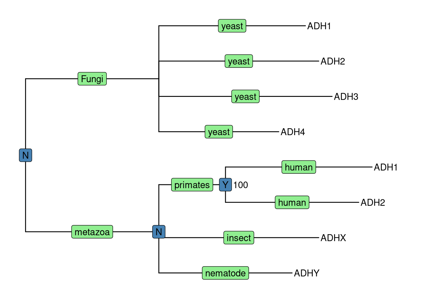
Figure 5.1: Annotating tree using grammar of graphics. The NHX tree was annotated using grammar of graphic syntax by combining different layers using + operator. Species information were labelled on the middle of the branches, Duplication events were shown on most recent common ancestor and clade bootstrap value were dispalyed near to it.
Here, as an example, we visualized the tree with several layers to display annotation stored in NHX tags, including a layer of geom_tiplab to display tip labels (gene name in this case), a layer using geom_label to show species information (S tag) colored by lightgreen, a layer of duplication event information (D tag) colored by steelblue and another layer using geom_text to show bootstrap value (B tag).
Layers defined in ggplot2 can be applied to ggtree directly as demonstrated in Figure 5.1 of using geom_label and geom_text. But ggplot2 does not provide graphic layers that are specific designed for phylogenetic tree annotation. For instance, layers for tip labels, tree branch scale legend, highlight or labeling clade are all unavailable. To make tree annotation more flexible, a number of layers have been implemented in ggtree (Table 5.1), enabling different ways of annotation on various parts/components of a phylogenetic tree.
| Layer | Description |
|---|---|
| geom_balance | highlights the two direct descendant clades of an internal node |
| geom_cladelabel | annotate a clade with bar and text label |
| geom_facet | plot associated data in specific panel (facet) and align the plot with the tree |
| geom_hilight | highlight selected clade with rectanglar or round shape |
| geom_inset | add insets (subplots) to tree nodes |
| geom_label2 | modified version of geom_label, with subsetting supported |
| geom_nodepoint | annotate internal nodes with symbolic points |
| geom_point2 | modified version of geom_point, with subsetting supported |
| geom_range | bar layer to present uncertainty of evolutionary inference |
| geom_rootpoint | annotate root node with symbolic point |
| geom_rootedge | add root edge to a tree |
| geom_segment2 | modified version of geom_segment, with subsetting supported |
| geom_strip | annotate associated taxa with bar and (optional) text label |
| geom_taxalink | Linking related taxa |
| geom_text2 | modified version of geom_text, with subsetting supported |
| geom_tiplab | layer of tip labels |
| geom_tippoint | annotate external nodes with symbolic points |
| geom_tree | tree structure layer, with multiple layout supported |
| geom_treescale | tree branch scale legend |
5.2 Layers for Tree Annotation
5.2.1 Colored strips
ggtree (Yu et al. 2017) implements geom_cladelabel layer to annotate a selected clade with a bar indicating the clade with a corresponding label.
The geom_cladelabel layer accepts a selected internal node number and label corresponding clade automatically (Figure 5.2A). To get the internal node number, please refer to Chapter 2.
set.seed(2015-12-21)
tree <- rtree(30)
p <- ggtree(tree) + xlim(NA, 6)

p + geom_cladelabel(node=45, label="test label") +
    geom_cladelabel(node=34, label="another clade")
Users can set the parameter, align = TRUE, to align the clade label, offset, to adjust the position and color to set the color of bar and label text etc (Figure 5.2B).
p + geom_cladelabel(node=45, label="test label", align=TRUE,  offset = .2, color='red') +
    geom_cladelabel(node=34, label="another clade", align=TRUE, offset = .2, color='blue')
Users can change the angle of the clade label text and relative position from text to bar via the parameter offset.text. The size of the bar and text can be changed via the parameters barsize and fontsize respectively (Figure 5.2C).
p + geom_cladelabel(node=45, label="test label", align=T, angle=270, hjust='center', offset.text=.5, barsize=1.5) +
    geom_cladelabel(node=34, label="another clade", align=T, angle=45, fontsize=8)
Users can also use geom_label to label the text and can set the background color by fill parameter (Figure 5.2D).
p + geom_cladelabel(node=34, label="another clade", align=T, geom='label', fill='lightblue')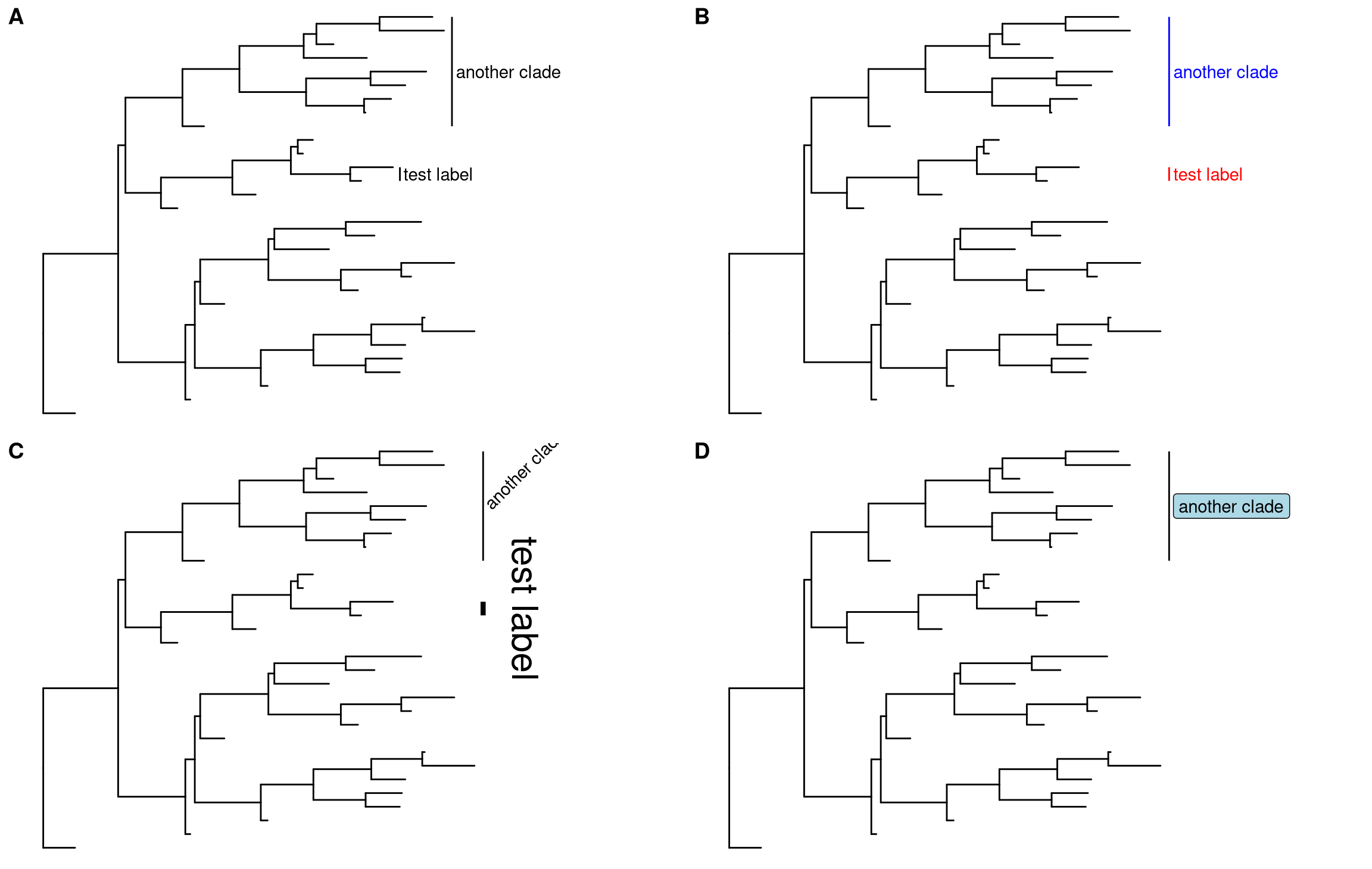
Figure 5.2: Labeling clades.
geom_cladelabel also supports unrooted tree layouts (Figure 5.3A).
ggtree(tree, layout="daylight") +
  geom_cladelabel(node=35, label="test label", angle=0,
                  fontsize=8, offset=.5, vjust=.5)  +
  geom_cladelabel(node=55, label='another clade',
                  angle=-95, hjust=.5, fontsize=8)
geom_cladelabel is designed for labeling Monophyletic (Clade) while there are related taxa that are not form a clade. ggtree provides geom_strip to add a strip/bar to indicate the association with optional label for Polyphyletic or Paraphyletic (Figure 5.3B).
p + geom_tiplab() +
  geom_strip('t10', 't30', barsize=2, color='red',
            label="associated taxa", offset.text=.1) +
  geom_strip('t1', 't18', barsize=2, color='blue',
            label = "another label", offset.text=.1)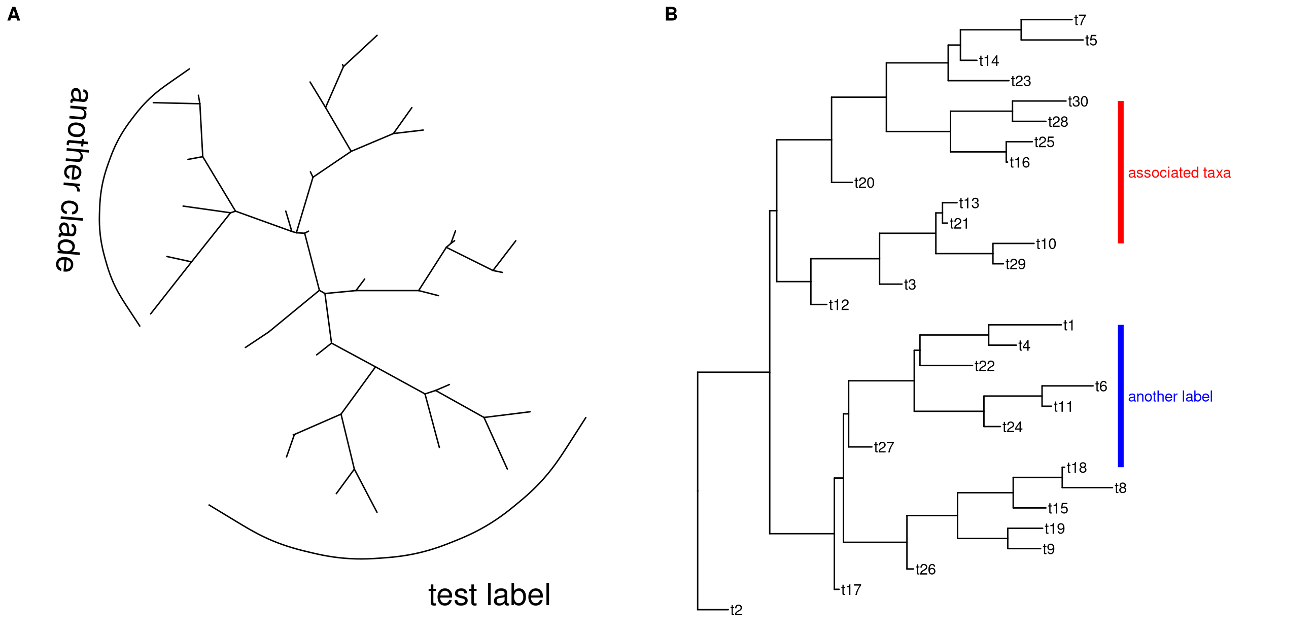
Figure 5.3: Labeling associated taxa. geom_cladelabel is for labeling Monophyletic and it also supports unrooted layout (A). geom_strip is designed for labeling associated taxa (Monophyletic, Polyphyletic or Paraphyletic) (B).
5.2.2 Highlight clades
ggtree implements geom_hilight layer, that accepts an internal node number and add a layer of rectangle to highlight the selected clade Figure (5.4).12
nwk <- system.file("extdata", "sample.nwk", package="treeio")
tree <- read.tree(nwk)
ggtree(tree) + geom_hilight(node=21, fill="steelblue", alpha=.6) +
geom_hilight(node=17, fill="darkgreen", alpha=.6) ggtree(tree, layout="circular") + geom_hilight(node=21, fill="steelblue", alpha=.6) +
geom_hilight(node=23, fill="darkgreen", alpha=.6)The geom_hilight layer also support highlighting clades for unrooted layout trees with round (‘encircle’) or rectangular (‘rect’) shape (Figure 5.4C).
## type can be 'encircle' or 'rect'
pg + geom_hilight(node=55) +
  geom_hilight(node=35, fill='darkgreen', type="rect")
Another way to highlight selected clades is setting the clades with different colors and/or line types as demonstrated in Figure 6.2.
In addition to geom_hilight, ggtree also implements geom_balance
which is designed to highlight neighboring subclades of a given internal node (Figure 5.4D).
ggtree(tree) +
  geom_balance(node=16, fill='steelblue', color='white', alpha=0.6, extend=1) +
  geom_balance(node=19, fill='darkgreen', color='white', alpha=0.6, extend=1)
The geom_hilight layer supports using aesthetic mapping to automatically highlight clades as demonstrated in Figure 5.4E and 5.4F.
## using external data
d <- data.frame(node=c(17, 21), type=c("A", "B"))
ggtree(tree) + geom_hilight(data=d, aes(node=node, fill=type))

## using data stored in tree object
x <- read.nhx(system.file("extdata/NHX/ADH.nhx", package="treeio"))
ggtree(x) + geom_hilight(mapping=aes(subset = node %in% c(10, 12), fill = S)) +
  scale_fill_manual(values=c("steelblue", "darkgreen"))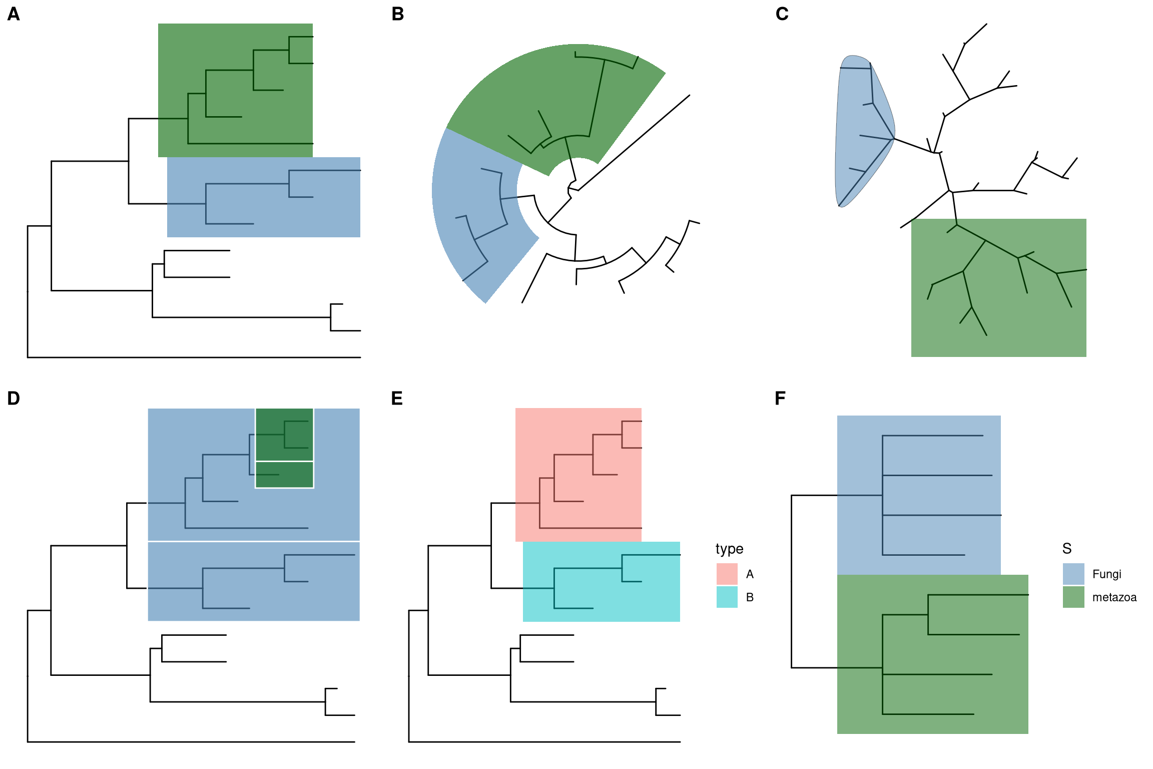
Figure 5.4: Highlight selected clades. Rectangular layout (A), circular/fan (B) and unrooted layouts. Highlight neighboring subclades simultaneously (D). Highlight selected clades using associated data (E and F).
5.2.3 Taxa connection
Some evolutionary events (e.g. reassortment, horizontal gene transfer) cannot be modeled by a simple tree. ggtree provides geom_taxalink layer that allows drawing straight or curved lines between any of two nodes in the tree, allow it to represent evolutionary events by connecting taxa. It works with rectangular (Figure 5.5A), circular (Figure 5.5B) and inward circular (Figure 5.5C) layouts.
The geom_taxalink layout supports aesthetic mapping, which requires a data.frame that stored association information with/without meta data as input (Figure 5.5D).
p1 <- ggtree(tree) + geom_tiplab() + geom_taxalink(taxa1='A', taxa2='E') +
  geom_taxalink(taxa1='F', taxa2='K', color='red', linetype = 'dashed',
    arrow=arrow(length=unit(0.02, "npc")))

p2 <- ggtree(tree, layout="circular") +
      geom_taxalink(taxa1='A', taxa2='E', color="grey", alpha=0.5, offset=0.05,
                    arrow=arrow(length=unit(0.01, "npc"))) +
      geom_taxalink(taxa1='F', taxa2='K', color='red', linetype = 'dashed', alpha=0.5, offset=0.05,
                    arrow=arrow(length=unit(0.01, "npc"))) +
      geom_taxalink(taxa1="L", taxa2="M", color="blue", alpha=0.5, offset=0.05,
                    hratio=0.8, arrow=arrow(length=unit(0.01, "npc"))) +
      geom_tiplab()

# when the tree was created using reverse x,
# we can set outward to FALSE, which will generate the inward curve lines.
p3 <- ggtree(tree, layout="inward_circular", xlim=150) +
      geom_taxalink(taxa1='A', taxa2='E', color="grey", alpha=0.5, offset=-0.2,
                    outward=FALSE,
                    arrow=arrow(length=unit(0.01, "npc"))) +
      geom_taxalink(taxa1='F', taxa2='K', color='red', linetype = 'dashed', alpha=0.5, offset=-0.2,
                    outward=FALSE,
                    arrow=arrow(length=unit(0.01, "npc"))) +
      geom_taxalink(taxa1="L", taxa2="M", color="blue", alpha=0.5, offset=-0.2,
                    outward=FALSE,
                    arrow=arrow(length=unit(0.01, "npc"))) +
      geom_tiplab(hjust=1)

dat <- data.frame(from=c("A", "F", "L"),
                  to=c("E", "K", "M"),
                  h=c(1, 1, 0.1),
                  type=c("t1", "t2", "t3"),
                  s=c(2, 1, 2))
p4 <- ggtree(tree, layout="inward_circular", xlim=c(150, 0)) +
          geom_taxalink(data=dat,
                         mapping=aes(taxa1=from,
                                     taxa2=to,
                                     color=type,
                                     size=s),
                         ncp=10,
                         offset=0.15) +
          geom_tiplab(hjust=1) +
          scale_size_continuous(range=c(1,3))
cowplot::plot_grid(p1, p2, p3, p4, ncol=2, labels=LETTERS[1:4])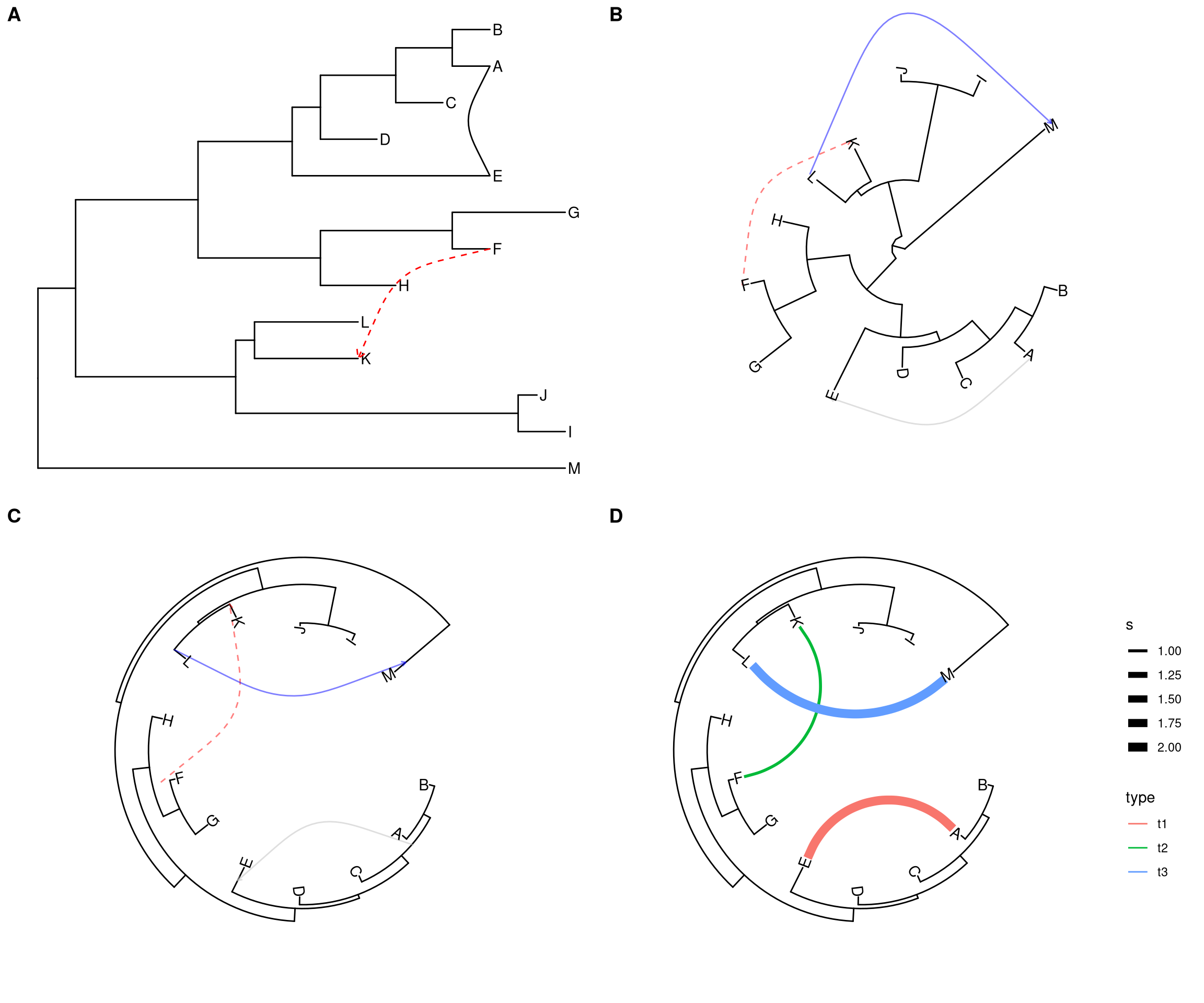
Figure 5.5: Linking related taxa. This can be used to indicate evolutionary events such as reassortment and horizontal gene transfer.
5.2.4 Uncertainty of evolutionary inference
The geom_range layer supports displaying interval (highest posterior density, confidence interval, range) as horizontal bars on tree nodes. The center of the interval will anchor to corresponding node. The center by default is the mean value of the interval (Figure 5.6A). We can set the center to estimated mean or median value (Figure 5.6B), or observed value. As the tree branch and the interval may not be in the same scale, ggtree provides scale_x_range to add second x axis for the range (Figure 5.6C). Note that x axis is disable by default theme and we need to enable it if we want to dispaly it (e.g. theme_tree2).
file <- system.file("extdata/MEGA7", "mtCDNA_timetree.nex", package = "treeio")
x <- read.mega(file)
p1 <- ggtree(x) + geom_range('reltime_0.95_CI', color='red', size=3, alpha=.3)
p2 <- ggtree(x) + geom_range('reltime_0.95_CI', color='red', size=3, alpha=.3, center='reltime')
p3 <- p2 + scale_x_range() + theme_tree2()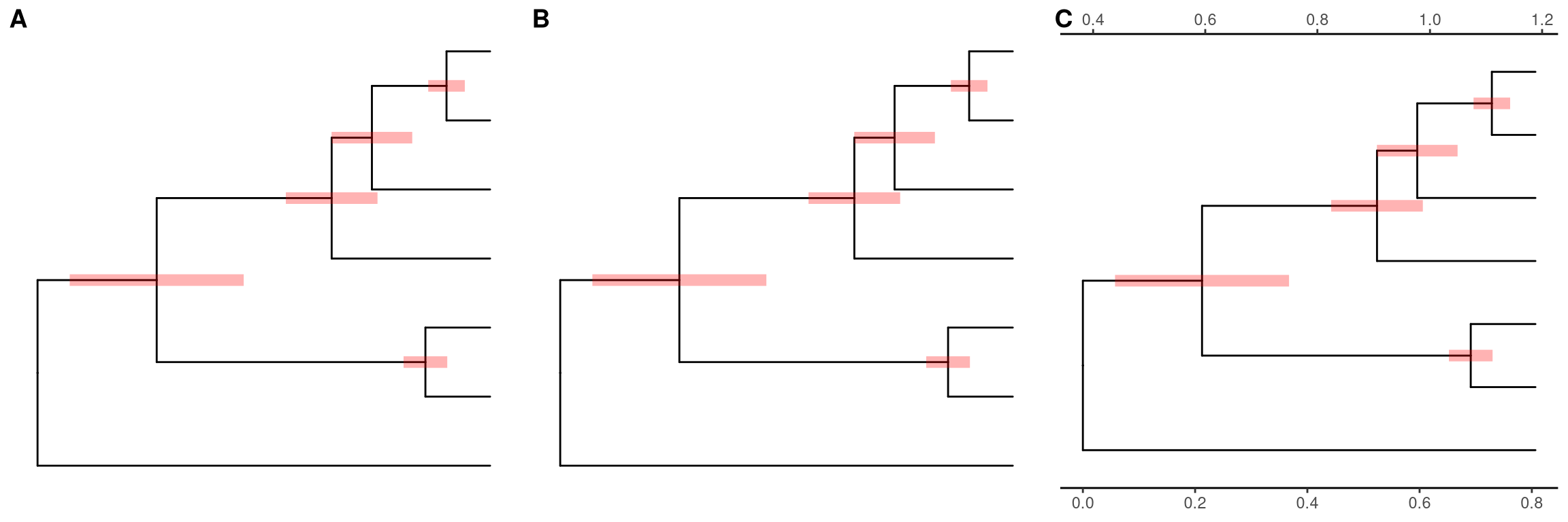
Figure 5.6: Displaying uncertainty of evolutoinary inference. The center (mean value of the range (A) or estimated value (B)) is anchor to the tree nodes. A second x axis was used for range scaling (C).
5.3 Tree annotation with output from evolution software
5.3.1 Tree annotation using data from evolutionary analysis software
Chapter 1 introduced using treeio packages to parse different tree formats and commonly used software outputs to obtain phylogeny-associated data. These imported data as S4 objects can be visualized directly using ggtree. Figure 5.1 demonstrates a tree annotated using the information (species classification, duplication event and bootstrap value) stored in NHX file. PHYLDOG and RevBayes output NHX files that can be parsed by treeio and visualized by ggtree with annotation using their inference data.
Furthermore, the evolutionary data from the inference of BEAST, MrBayes and RevBayes, dN/dS values inferred by CodeML, ancestral sequences inferred by HyPhy, CodeML or BaseML and short read placement by EPA and pplacer can be used to annotate the tree directly.
file <- system.file("extdata/BEAST", "beast_mcc.tree", package="treeio")
beast <- read.beast(file)
ggtree(beast, aes(color=rate))  +
    geom_range(range='length_0.95_HPD', color='red', alpha=.6, size=2) +
    geom_nodelab(aes(x=branch, label=round(posterior, 2)), vjust=-.5, size=3) +
    scale_color_continuous(low="darkgreen", high="red") +
    theme(legend.position=c(.1, .8))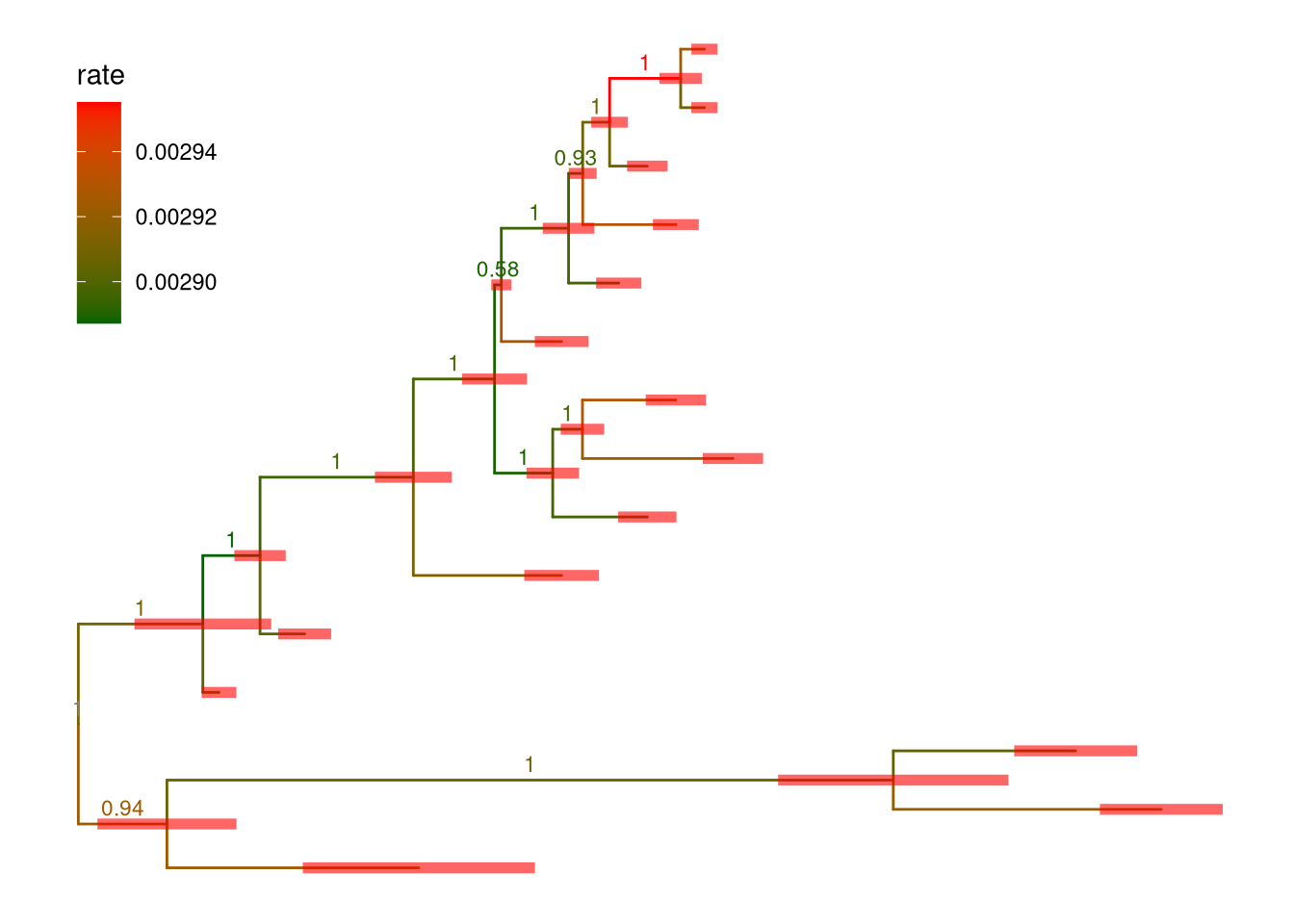
Figure 5.7: Annotating BEAST tree with length_95%_HPD and posterior. Branch length credible intervals (95% HPD) were displayed as red horizontal bars and clade posterior values were shown on the middle of branches.
In Figure 5.7, the tree was visualized and annotated with posterior > 0.9 and demonstrated length uncertainty (95% Highest Posterior Density (HPD) interval).
Ancestral sequences inferred by HyPhy can be parsed using treeio, whereas the substitutions along each tree branch was automatically computed and stored inside the phylogenetic tree object (i.e., S4 object). The ggtree can utilize this information in the object to annotate the tree, as demonstrated in Figure 5.8.
nwk <- system.file("extdata/HYPHY", "labelledtree.tree",
                   package="treeio")
ancseq <- system.file("extdata/HYPHY", "ancseq.nex",
                      package="treeio")
tipfas <- system.file("extdata", "pa.fas", package="treeio")
hy <- read.hyphy(nwk, ancseq, tipfas)
ggtree(hy) +
  geom_text(aes(x=branch, label=AA_subs), size=2,
            vjust=-.3, color="firebrick")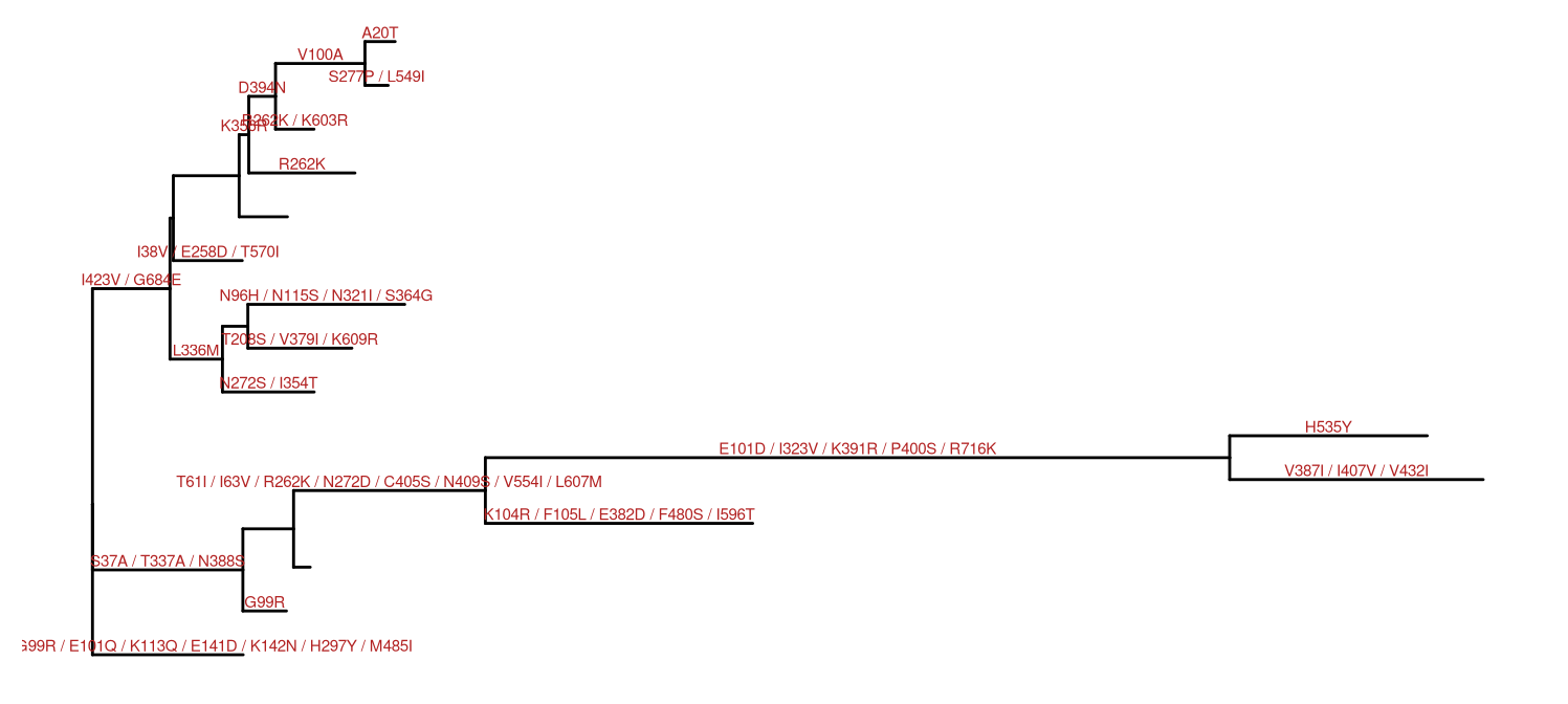
Figure 5.8: Annotating tree with amino acid substitution determined by ancestral sequences inferred by HYPHY. Amino acid substitutions were displayed on the middle of branches.
PAML’s BaseML and CodeML can be also used to infer ancestral sequences, whereas CodeML can infer selection pressure. After parsing this information using treeio, ggtree can integrate this information into the same tree structure and used for annotation as illustrated in Figure 5.9.
rstfile <- system.file("extdata/PAML_Codeml", "rst",
                       package="treeio")
mlcfile <- system.file("extdata/PAML_Codeml", "mlc",
                       package="treeio")
ml <- read.codeml(rstfile, mlcfile)
ggtree(ml, aes(color=dN_vs_dS), branch.length='dN_vs_dS') +
  scale_color_continuous(name='dN/dS', limits=c(0, 1.5),
                         oob=scales::squish,
                         low='darkgreen', high='red') +
  geom_text(aes(x=branch, label=AA_subs),
            vjust=-.5, color='steelblue', size=2) +
  theme_tree2(legend.position=c(.9, .3))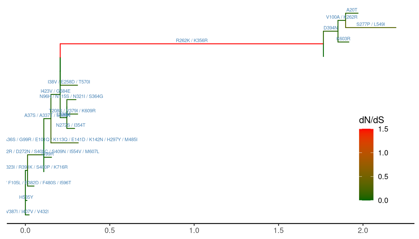
Figure 5.9: Annotating tree with animo acid substitution and dN/dS inferred by CodeML. Branches were rescaled and colored by dN/dS values and amino acid substitutions were displayed on the middle of branches.
Not only all the tree data that parsed by treeio can be used to visualize and annotate phylogenetic tree using ggtree, but also other tree and tree-like objects defined in R community are supported. The ggtree plays an unique role in R ecosystem to facilitate phylogenetic analysis and it can be easily integrated into other packages and pipelines. For more details, please refer to chapter 9. In addition to direct support of tree objects, ggtree also allow users to plot tree with different types of external data (see also chapter 7 and (Yu et al. 2018)).
5.4 Summary
ggtree implements grammar of graphics for annotating phylogenetic trees. Users can use ggplot2 syntax to combine different annotation layers to produce complex tree annotation. If you are familiar with ggplot2, tree annotation with high level of customization can be intuitive and flexible using ggtree.
References
Yu, Guangchuang, Tommy Tsan-Yuk Lam, Huachen Zhu, and Yi Guan. 2018. “Two Methods for Mapping and Visualizing Associated Data on Phylogeny Using Ggtree.” Molecular Biology and Evolution 35 (12): 3041–3. https://doi.org/10.1093/molbev/msy194.
Yu, Guangchuang, David K. Smith, Huachen Zhu, Yi Guan, and Tommy Tsan-Yuk Lam. 2017. “Ggtree: An R Package for Visualization and Annotation of Phylogenetic Trees with Their Covariates and Other Associated Data.” Methods in Ecology and Evolution 8 (1): 28–36. https://doi.org/10.1111/2041-210X.12628.