Chapter 10 ggtreeExtra
10.1 Introduction
Phylogenetic trees can be easily visualized with multiple layout using ggtree (Yu et al. 2017). It provides programmable visualization and annotation of phylogenetic trees. It not only supports visualization and annotation of phylogenetic trees but also other tree-like structures. So it can be generally applied in related biological researches. None R package, to our knowledge, are developed to align multiple layers to the circular trees or other layout trees. To solve the problem, We developed ggtreeExtra, which can align associated graphs to circular, fan or radial and other rectangular layout tree. ggtreeExtra provides function, geom_fruit to align graphs to the tree. But the associated graphs will align in different position. So we also developed geom_fruit_list to add multiple layers in the same position. Furthermore, The axis of external layers can be added using the axis.params=list(add.axis=TRUE) in geom_fruit. The grid lines of external layers can be added using the grid.params=list(add.grid=TRUE) in geom_fruit. These functions are based on ggplot2 using grammar of graphics (Wickham 2009).
10.2 Aligning graphs to the tree based on tree structure
The phylogenetic trees are often visualized with different graph created using associated datasets. Like the geom_facet of ggtree (Yu et al. 2017), ggtreeExtra also provides geom_fruit layer which accepts an input data.frame and a geom function to plot the input data. The data will be visualized in an additional position of the plot. geom_fruit also is a general function to link graphs to phylogenetic trees. It will re-orders the input data based on the tree structure and displayed the data with the associated geom at specific position.
The geom_fruit is designed to work with most of geom layers defined in ggplot2. It control the position of graphs by position parameter, which was provided the Position object of ggtreeExtra. The default position parameters is ‘auto’. This means that the geom_bar will use position_stackx(), geom_violin and geom_boxplot will use position_dodgex(), geom_point and geom_tile will use position_identityx(). So if the geom defined in other ggplot2-based packages has position parameter, which support the result of a call to a position adjustment function, it also can work with geom_fruit, such as geom_star in ggstar, which provides the regular polygon layer for easily discernible shapes based on the grammar of ggplot2. Since the ggplot2 community keeps expanding and more geom layers will be implemented in either ggplot2 or other extensions, geom_fruit also will gain more power to present data in future.
library(ggtreeExtra)
library(ggtree)
library(phyloseq)
library(dplyr)

data("GlobalPatterns")
GP <- GlobalPatterns
GP <- prune_taxa(taxa_sums(GP) > 600, GP)
sample_data(GP)$human <- get_variable(GP, "SampleType") %in%
                              c("Feces", "Skin")
mergedGP <- merge_samples(GP, "SampleType")
mergedGP <- rarefy_even_depth(mergedGP,rngseed=394582)
mergedGP <- tax_glom(mergedGP,"Order")

melt_simple <- psmelt(mergedGP) %>%
               filter(Abundance < 120) %>%
               select(OTU, val=Abundance)

p <- ggtree(mergedGP, layout="fan", open.angle=30) +
     geom_tippoint(mapping=aes(color=Phylum),
                   size=1.5,
                   show.legend=FALSE)

p <- p +
     geom_fruit(
         data=melt_simple,
         geom=geom_boxplot,
         mapping = aes(
                     y=OTU,
                     x=val,
                     group=label,
                     fill=Phylum,
                   ),
         lwd=.2,
         outlier.size=0.5,
         outlier.stroke=0.08,
         outlier.shape=21,
         axis.params=list(
                         add.axis   =TRUE,
                         text.angle =-45,
                         text.size  = 4,
                         hjust      = 0,
                         vjust      = 0.5
                     ),
         grid.params=list(
                         add.grid=TRUE
                     )
     ) +
     scale_fill_manual(
         name="Phyla",
         values=scales::hue_pal()(24),
         guide=guide_legend(keywidth=0.8, keyheight=0.8, ncol=1)
     ) +
     theme(
         legend.title=element_text(size=20),
         legend.text=element_text(size=15)
     )
p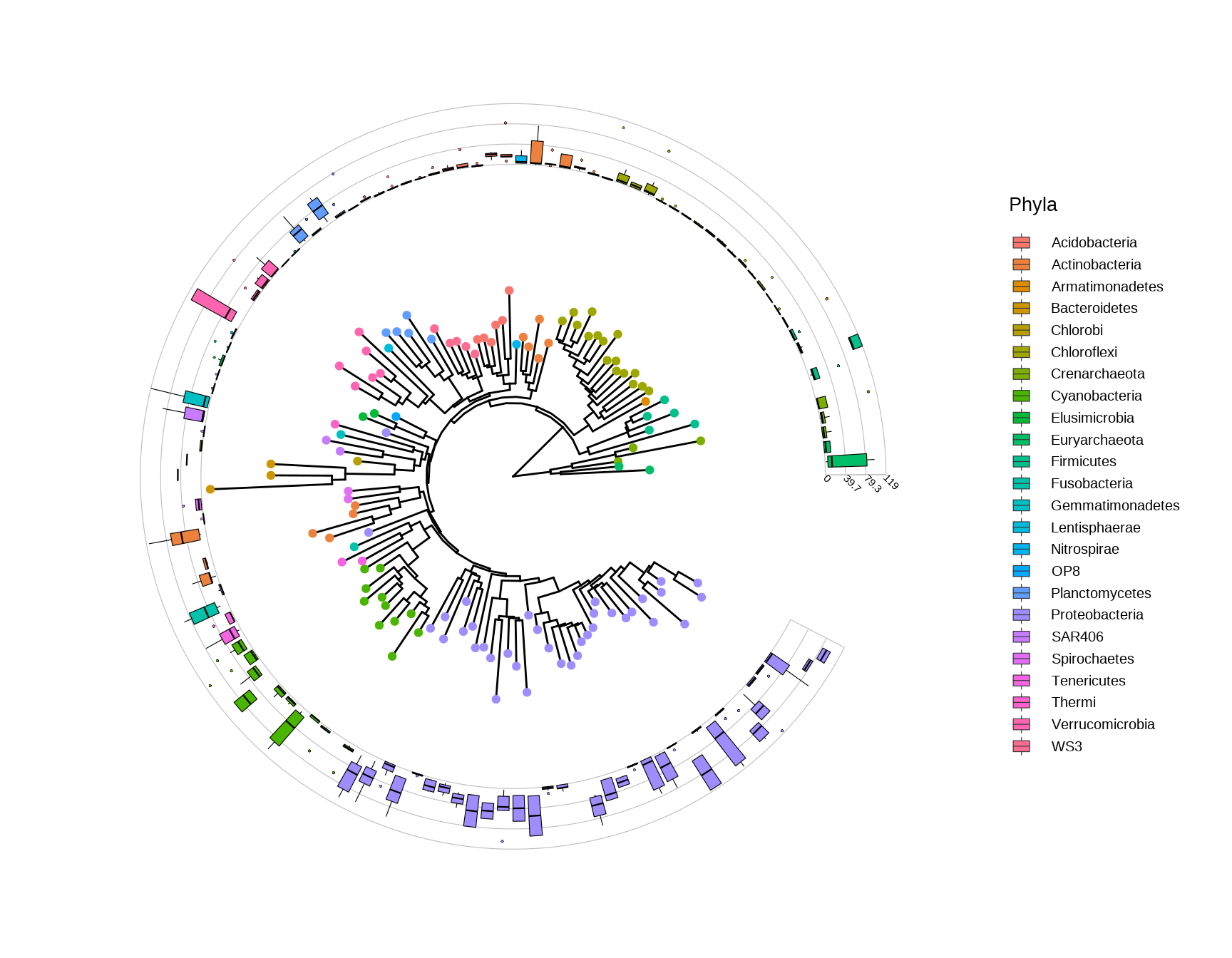
Figure 10.1: Phylogenetic tree with OTU abundance distribution.
This example uses microbiome data that provided in phyloseq package and boxplot is employed to visualize species abundance data. The geom_fruit layer automatically re-arranges the abundance data according to the circular tree structure, visualizes the data using the specify geom function.
10.3 Aligning multiple graphs to the tree for multi-dimensional data
Circular layout is efficient layout to show the phylogenetic tree and multi-dimensional data. The continuous dataset can be displayed using heat map, bar plot, box plot or dot plot etc. This example reproduce Fig.2 of (Morgan, Segata, and Huttenhower 2013). The data is provided by GraPhlAn (Asnicar et al. 2015), which contained the relative abundance of microbiome at different body sites. This example demonstrates the abilities of adding multiple layers (dot plot, heat map and bar plot) created with continuous data to a specific panel, and the attributes of tip point also can be extracted to map Figure 10.2.
library(ggtreeExtra)
library(ggtree)
library(treeio)
library(tidytree)
library(ggstar)
library(ggplot2)
library(ggnewscale)

tree <- read.tree("data/HMP_tree/hmptree.nwk")
# the abundance and types of microbes
dat1 <- read.csv("data/HMP_tree/tippoint_attr.csv")
# the abundance of microbes at different body sites.
dat2 <- read.csv("data/HMP_tree/ringheatmap_attr.csv")
# the abundance of microbes at the body sites of greatest prevalence.
dat3 <- read.csv("data/HMP_tree/barplot_attr.csv")

# adjust the order
dat2$Sites <- factor(dat2$Sites, levels=c("Stool (prevalence)", "Cheek (prevalence)",
                                          "Plaque (prevalence)","Tongue (prevalence)",
                                          "Nose (prevalence)", "Vagina (prevalence)",
                                          "Skin (prevalence)"))
dat3$Sites <- factor(dat3$Sites, levels=c("Stool (prevalence)", "Cheek (prevalence)",
                                          "Plaque (prevalence)", "Tongue (prevalence)",
                                          "Nose (prevalence)", "Vagina (prevalence)",
                                          "Skin (prevalence)"))
# extract the clade label information. Because some nodes of tree are annotated to genera,
# which can be displayed with high light using ggtree.
nodeids <- nodeid(tree, tree$node.label[nchar(tree$node.label)>4])
nodedf <- data.frame(node=nodeids)
nodelab <- gsub("[\\.0-9]", "", tree$node.label[nchar(tree$node.label)>4])
# The layers of clade and hightlight
hightlight <- lapply(nodeids, function(x)geom_hilight(node=x, extendto=6.8, alpha=0.3,
                                                      fill="grey", color="grey50", size=0.05))
poslist <- c(1.6, 1.4, 1.6, 0.8, 0.1, 0.25, 1.6, 1.6, 1.2, 0.4,
             1.2, 1.8, 0.3, 0.8, 0.4, 0.3, 0.4, 0.4, 0.4, 0.6,
             0.3, 0.4, 0.3)
cladelabels <- mapply(function(x, y, z){geom_cladelabel(node=x, label=y, barsize=NA, extend=0,
                                                    offset.text=z, fontsize=10, angle="auto",
                                                    hjust=0.5, horizontal=FALSE, fontface="italic")},
                                     nodeids, nodelab, poslist, SIMPLIFY=FALSE)

# The circular layout tree.
p <- ggtree(tree, layout="fan", size=0.15, open.angle=5) +
     geom_hilight(data=nodedf, mapping=aes(node=node),
                  extendto=6.8, alpha=0.3, fill="grey", color="grey50",
                  size=0.05)
p <- p %<+% dat1 + geom_fruit(geom=geom_star,
                              mapping=aes(fill=Phylum, starshape=Type, size=Size),
                              position="identity",starstroke=0.1)+
         scale_fill_manual(values=c("#FFC125","#87CEFA","#7B68EE","#808080","#800080",
                                    "#9ACD32","#D15FEE","#FFC0CB","#EE6A50","#8DEEEE",
                                    "#006400","#800000","#B0171F","#191970"),
                           guide=guide_legend(keywidth = 0.5, keyheight = 0.5, order=1,
                                              override.aes=list(starshape=15)),
                           na.translate=FALSE)+
         scale_starshape_manual(values=c(15, 1),
                                guide=guide_legend(keywidth = 0.5, keyheight = 0.5, order=2),
                                na.translate=FALSE)+
         scale_size_continuous(range = c(1, 2.5),
                               guide = guide_legend(keywidth = 0.5, keyheight = 0.5, order=3,
                                                    override.aes=list(starshape=15)))+
         new_scale_fill()+
         geom_fruit(data=dat2, geom=geom_tile,
                    mapping=aes(y=ID, x=Sites, alpha=Abundance, fill=Sites),
                    color = "grey50", offset = 0.04,size = 0.02)+
         scale_alpha_continuous(range=c(0, 1),
                             guide=guide_legend(keywidth = 0.3, keyheight = 0.3, order=5)) +
         cladelabels +
         geom_fruit(data=dat3, geom=geom_bar,
                    mapping=aes(y=ID, x=HigherAbundance, fill=Sites),
                    pwidth=0.38,
                    orientation="y",
                    stat="identity",
         )+
         scale_fill_manual(values=c("#0000FF","#FFA500","#FF0000","#800000",
                                    "#006400","#800080","#696969"),
                           guide=guide_legend(keywidth = 0.3, keyheight = 0.3, order=4))+
         geom_treescale(fontsize=8, linesize=0.3, x=4.9, y=0.1) +
         theme(legend.position=c(0.93, 0.5),
               legend.background=element_rect(fill=NA),
               legend.title=element_text(size=40),
               legend.text=element_text(size=30),
               legend.spacing.y = unit(0.02, "cm"),
             )
p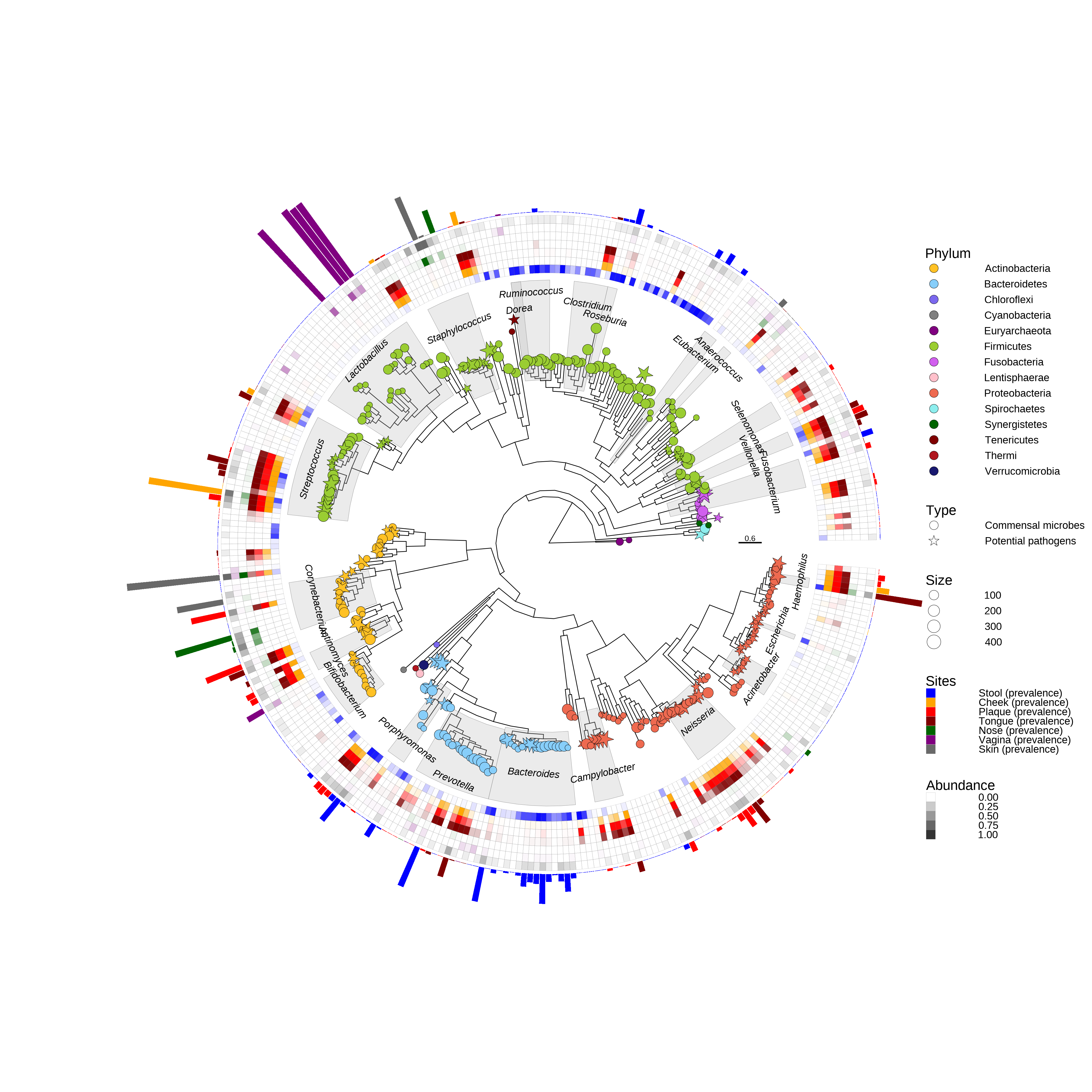
Figure 10.2: Phylogenetic tree about the abundance of microbes at different sites of human.
The shape of tip labels indicated the commensal microbes or potential pathogens. The transparency of heat map indicates the abundance of microbes, and colors of heat map indicate the different sites of human. The bar plot indicates the relative abundance at body site of the most abundance. The node labels contain taxonomy information in this example, so it can be highlight using geom_hilight. The datasets disabled with heat map and bar plot are the format of specific geom of ggplot2. If you have short table format datasets, you can use reshape2::melt() or tidyr::pivot_longer() to convert them.
References
Asnicar, Francesco, George Weingart, Timothy L Tickle, Curtis Huttenhower, and Nicola Segata. 2015. “Compact Graphical Representation of Phylogenetic Data and Metadata with Graphlan.” PeerJ 3: e1029. https://doi.org/10.7717/peerj.1029.
Morgan, Xochitl C., Nicola Segata, and Curtis Huttenhower. 2013. “Biodiversity and Functional Genomics in the Human Microbiome.” Trends in Genetics 29 (1): 51–58. https://doi.org/10.1016/J.TIG.2012.09.005.
Wickham, Hadley. 2009. Ggplot2: Elegant Graphics for Data Analysis. 1st ed. Springer.
Yu, Guangchuang, David K. Smith, Huachen Zhu, Yi Guan, and Tommy Tsan-Yuk Lam. 2017. “Ggtree: An R Package for Visualization and Annotation of Phylogenetic Trees with Their Covariates and Other Associated Data.” Methods in Ecology and Evolution 8 (1): 28–36. https://doi.org/10.1111/2041-210X.12628.