Interpolate MEG or EEG data to any montage

This example demonstrates both EEG montage interpolation and MEG system transformation.

For EEG, this can be useful for standardizing EEG channel layouts across different datasets (see [1]).

• Using the field interpolation for EEG data.

• Using the target montage “biosemi16”.

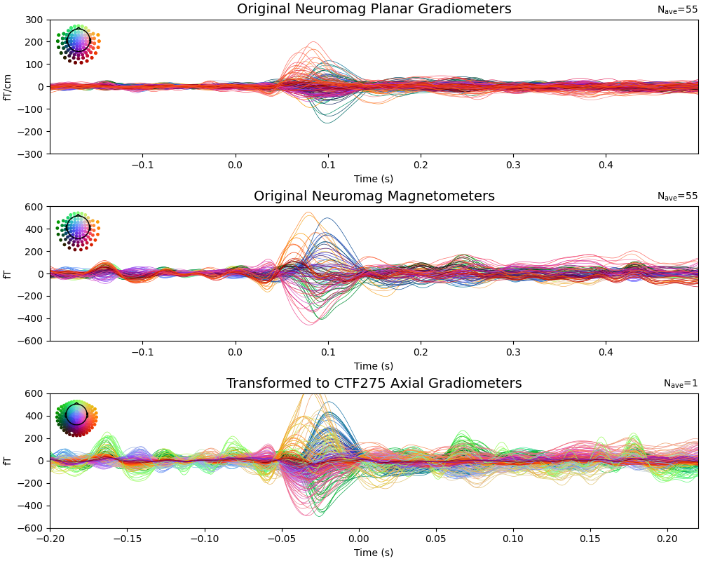
• Using the MNE interpolation for MEG data to transform from Neuromag (planar gradiometers and magnetometers) to CTF (axial gradiometers).

In the first example, the data from the original EEG channels will be interpolated onto the positions defined by the “biosemi16” montage.

In the second example, we will interpolate MEG data from a 306-sensor Neuromag to 275-sensor CTF system.

# Authors: Antoine Collas <contact@antoinecollas.fr>
#          Konstantinos Tsilimparis <konstantinos.tsilimparis@outlook.com>
# License: BSD-3-Clause
# Copyright the MNE-Python contributors.

import matplotlib.pyplot as plt

import mne
from mne.channels import make_standard_montage
from mne.datasets import sample

print(__doc__)
ylim = (-10, 10)

Part 1: EEG System Transformation

# Load EEG data
data_path = sample.data_path()
eeg_file_path = data_path / "MEG" / "sample" / "sample_audvis-ave.fif"
evoked = mne.read_evokeds(eeg_file_path, condition="Left Auditory", baseline=(None, 0))

# Select only EEG channels
evoked.pick("eeg")

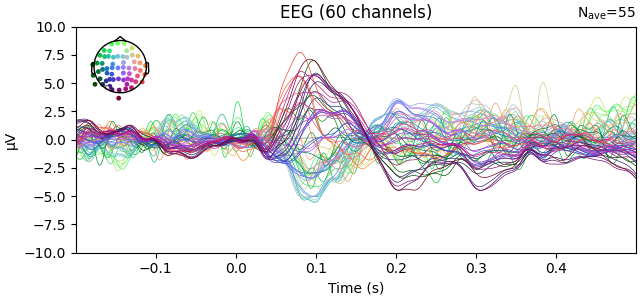
# Plot the original EEG layout
evoked.plot(exclude=[], picks="eeg", ylim=dict(eeg=ylim))

Reading /home/circleci/mne_data/MNE-sample-data/MEG/sample/sample_audvis-ave.fif ...
    Read a total of 4 projection items:
        PCA-v1 (1 x 102) active
        PCA-v2 (1 x 102) active
        PCA-v3 (1 x 102) active
        Average EEG reference (1 x 60) active
    Found the data of interest:
        t =    -199.80 ...     499.49 ms (Left Auditory)
        0 CTF compensation matrices available
        nave = 55 - aspect type = 100
Projections have already been applied. Setting proj attribute to True.
Applying baseline correction (mode: mean)

Define the target montage

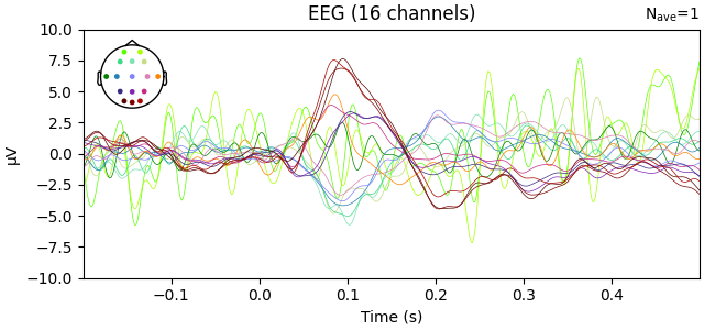
standard_montage = make_standard_montage("biosemi16")

Use interpolate_to to project EEG data to the standard montage

evoked_interpolated_spline = evoked.copy().interpolate_to(
    standard_montage, method="spline"
)

# Plot the interpolated EEG layout
evoked_interpolated_spline.plot(exclude=[], picks="eeg", ylim=dict(eeg=ylim))

Automatic origin fit: head of radius 91.2 mm

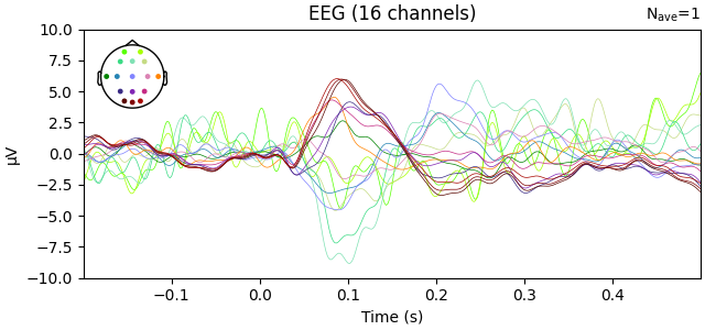
Use interpolate_to to project EEG data to the standard montage

evoked_interpolated_mne = evoked.copy().interpolate_to(standard_montage, method="MNE")

# Plot the interpolated EEG layout
evoked_interpolated_mne.plot(exclude=[], picks="eeg", ylim=dict(eeg=ylim))

Adding average EEG reference projection.
    Automatic origin fit: head of radius 91.2 mm
    Computing dot products for 59 EEG channels...
    Computing cross products for 59 → 16 EEG channels...
    Preparing the mapping matrix...
    Truncating at 58/59 components and regularizing with α=1.0e-01
    The map has an average electrode reference (16 channels)

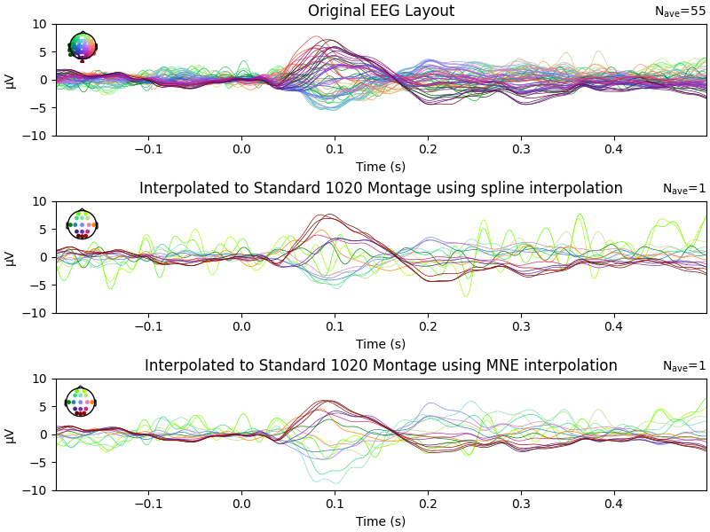
Comparing before and after interpolation

fig, axs = plt.subplots(3, 1, figsize=(8, 6), constrained_layout=True)
evoked.plot(exclude=[], picks="eeg", axes=axs[0], show=False, ylim=dict(eeg=ylim))
axs[0].set_title("Original EEG Layout")
evoked_interpolated_spline.plot(
    exclude=[], picks="eeg", axes=axs[1], show=False, ylim=dict(eeg=ylim)
)
axs[1].set_title("Interpolated to Standard 1020 Montage using spline interpolation")
evoked_interpolated_mne.plot(
    exclude=[], picks="eeg", axes=axs[2], show=False, ylim=dict(eeg=ylim)
)
axs[2].set_title("Interpolated to Standard 1020 Montage using MNE interpolation")

Part 2: MEG System Transformation

We demonstrate transforming MEG data from Neuromag (planar gradiometers and magnetometers) to CTF (axial gradiometers) sensor configuration.

# Load the full evoked data with MEG channels
evoked_meg = mne.read_evokeds(
    eeg_file_path, condition="Left Auditory", baseline=(None, 0)
)
evoked_meg.pick("meg")

print("Original Neuromag system:")
print(f"  Number of magnetometers: {len(mne.pick_types(evoked_meg.info, meg='mag'))}")
print(f"  Number of gradiometers: {len(mne.pick_types(evoked_meg.info, meg='grad'))}")

Reading /home/circleci/mne_data/MNE-sample-data/MEG/sample/sample_audvis-ave.fif ...
    Read a total of 4 projection items:
        PCA-v1 (1 x 102) active
        PCA-v2 (1 x 102) active
        PCA-v3 (1 x 102) active
        Average EEG reference (1 x 60) active
    Found the data of interest:
        t =    -199.80 ...     499.49 ms (Left Auditory)
        0 CTF compensation matrices available
        nave = 55 - aspect type = 100
Projections have already been applied. Setting proj attribute to True.
Applying baseline correction (mode: mean)
Original Neuromag system:
  Number of magnetometers: 102
  Number of gradiometers: 203

Transform to CTF sensor configuration

# Interpolate Neuromag to CTF
evoked_ctf = evoked_meg.copy().interpolate_to("ctf275", mode="accurate")

print("\nTransformed to CTF system:")
print(f"  Number of MEG channels: {len(mne.pick_types(evoked_ctf.info, meg=True))}")
print(f"  Bad channels in original: {evoked_meg.info['bads']}")

    Automatic origin fit: head of radius 91.2 mm
    Computing dot products for 305 MEG channels...
    Computing cross products for 305 → 274 MEG channels...
    Preparing the mapping matrix...
    Truncating at 85/305 components to omit less than 0.0001 (9.4e-05)

Transformed to CTF system:
  Number of MEG channels: 274
  Bad channels in original: ['MEG 2443']

Compare evoked responses: Original Neuromag vs Transformed CTF The data should be similar but projected onto different sensor arrays

# Set consistent y-limits for comparison
ylim_meg = dict(grad=[-300, 300], mag=[-600, 600], meg=[-300, 300])

fig, axes = plt.subplots(3, 1, figsize=(10, 8), layout="constrained")

# Plot original Neuromag gradiometers
evoked_meg.copy().pick("grad").plot(
    axes=axes[0], show=False, spatial_colors=True, ylim=ylim_meg, time_unit="s"
)
axes[0].set_title("Original Neuromag Planar Gradiometers", fontsize=14)


# Plot original Neuromag magnetometers
evoked_meg.copy().pick("mag").plot(
    axes=axes[1], show=False, spatial_colors=True, ylim=ylim_meg, time_unit="s"
)
axes[1].set_title("Original Neuromag Magnetometers", fontsize=14)

# Plot transformed CTF gradiometers
evoked_ctf.plot(
    axes=axes[2], show=False, spatial_colors=True, ylim=ylim_meg, time_unit="s"
)
axes[2].set_title("Transformed to CTF275 Axial Gradiometers", fontsize=14)

References

[1]

Apolline Mellot, Antoine Collas, Sylvain Chevallier, Denis Engemann, and Alexandre Gramfort. Physics-informed and unsupervised riemannian domain adaptation for machine learning on heterogeneous eeg datasets. In Proceedings of the 32nd European Signal Processing Conference (EUSIPCO). Lyon, France, 2024.