Note
Go to the end to download the full example code.
Generate simulated raw data#
This example generates raw data by repeating a desired source activation multiple times.
# Authors: Yousra Bekhti <yousra.bekhti@gmail.com>
#          Mark Wronkiewicz <wronk.mark@gmail.com>
#          Eric Larson <larson.eric.d@gmail.com>
#
# License: BSD-3-Clause
# Copyright the MNE-Python contributors.
import matplotlib.pyplot as plt
import numpy as np

import mne
from mne import Epochs, compute_covariance, find_events, make_ad_hoc_cov
from mne.datasets import sample
from mne.simulation import (
    add_ecg,
    add_eog,
    add_noise,
    simulate_raw,
    simulate_sparse_stc,
)

data_path = sample.data_path()
meg_path = data_path / "MEG" / "sample"
raw_fname = meg_path / "sample_audvis_raw.fif"
fwd_fname = meg_path / "sample_audvis-meg-eeg-oct-6-fwd.fif"

# Load real data as the template
raw = mne.io.read_raw_fif(raw_fname)
raw.set_eeg_reference(projection=True)
Opening raw data file /home/circleci/mne_data/MNE-sample-data/MEG/sample/sample_audvis_raw.fif...
    Read a total of 3 projection items:
        PCA-v1 (1 x 10²)  idle
        PCA-v2 (1 x 10²)  idle
        PCA-v3 (1 x 10²)  idle
    Range : 25800 ... 192599 =     42.956 ...   320.670 secs
Ready.
EEG channel type selected for re-referencing
Adding average EEG reference projection.
1 projection items deactivated
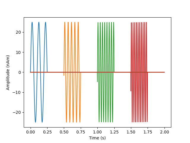
Generate dipole time series
n_dipoles = 4  # number of dipoles to create
epoch_duration = 2.0  # duration of each epoch/event
n = 0  # harmonic number
rng = np.random.RandomState(0)  # random state (make reproducible)


def data_fun(times):
    """Generate time-staggered sinusoids at harmonics of 10Hz."""
    global n
    n_samp = len(times)
    window = np.zeros(n_samp)
    start, stop = (
        int(ii * float(n_samp) / (2 * n_dipoles)) for ii in (2 * n, 2 * n + 1)
    )
    window[start:stop] = 1.0
    n += 1
    data = 25e-9 * np.sin(2.0 * np.pi * 10.0 * n * times)
    data *= window
    return data


times = raw.times[: int(raw.info["sfreq"] * epoch_duration)]
fwd = mne.read_forward_solution(fwd_fname)
src = fwd["src"]
stc = simulate_sparse_stc(
    src, n_dipoles=n_dipoles, times=times, data_fun=data_fun, random_state=rng
)
# look at our source data
fig, ax = plt.subplots(1)
ax.plot(times, 1e9 * stc.data.T)
ax.set(ylabel="Amplitude (nAm)", xlabel="Time (s)")
mne.viz.utils.plt_show()

Reading forward solution from /home/circleci/mne_data/MNE-sample-data/MEG/sample/sample_audvis-meg-eeg-oct-6-fwd.fif...
    Reading a source space...
    Computing patch statistics...
    Patch information added...
    Distance information added...
    [done]
    Reading a source space...
    Computing patch statistics...
    Patch information added...
    Distance information added...
    [done]
    2 source spaces read
    Desired named matrix (kind = 3523 (FIFF_MNE_FORWARD_SOLUTION_GRAD)) not available
    Read MEG forward solution (7498 sources, 306 channels, free orientations)
    Desired named matrix (kind = 3523 (FIFF_MNE_FORWARD_SOLUTION_GRAD)) not available
    Read EEG forward solution (7498 sources, 60 channels, free orientations)
    Forward solutions combined: MEG, EEG
    Source spaces transformed to the forward solution coordinate frame
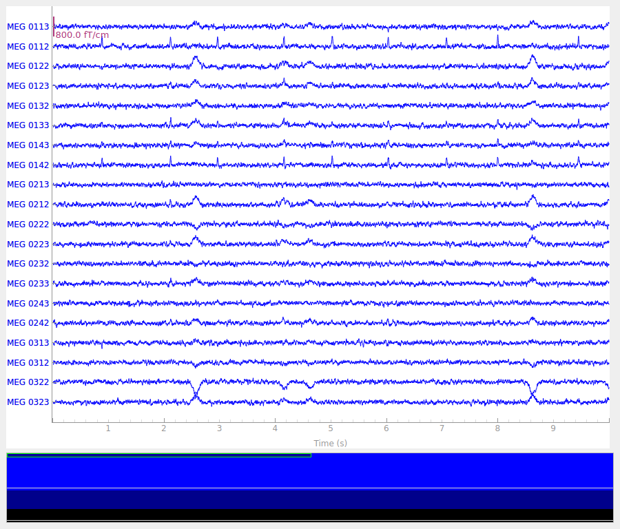
Simulate raw data
raw_sim = simulate_raw(raw.info, [stc] * 10, forward=fwd, verbose=True)
cov = make_ad_hoc_cov(raw_sim.info)
add_noise(raw_sim, cov, iir_filter=[0.2, -0.2, 0.04], random_state=rng)
add_ecg(raw_sim, random_state=rng)
add_eog(raw_sim, random_state=rng)
raw_sim.plot()

Setting up raw simulation: 1 position, "cos2" interpolation
Event information stored on channel:              STI 014
    Interval 0.000–2.000 s
Setting up forward solutions
Computing gain matrix for transform #1/1
    Interval 0.000–2.000 s
    Interval 0.000–2.000 s
    Interval 0.000–2.000 s
    Interval 0.000–2.000 s
    Interval 0.000–2.000 s
    Interval 0.000–2.000 s
    Interval 0.000–2.000 s
    Interval 0.000–2.000 s
    Interval 0.000–2.000 s
    10 STC iterations provided
[done]
Adding noise to 366/376 channels (366 channels in cov)
Sphere                : origin at (0.0 0.0 0.0) mm
              radius  : 0.1 mm
Source location file  : dict()
Assuming input in millimeters
Assuming input in MRI coordinates

Positions (in meters) and orientations
1 sources
ecg simulated and trace not stored
Setting up forward solutions
Computing gain matrix for transform #1/1
Sphere                : origin at (0.0 0.0 0.0) mm
              radius  : 0.1 mm
Source location file  : dict()
Assuming input in millimeters
Assuming input in MRI coordinates

Positions (in meters) and orientations
2 sources
blink simulated and trace stored on channel:      EOG 061
Setting up forward solutions
Computing gain matrix for transform #1/1
Using qt as 2D backend.
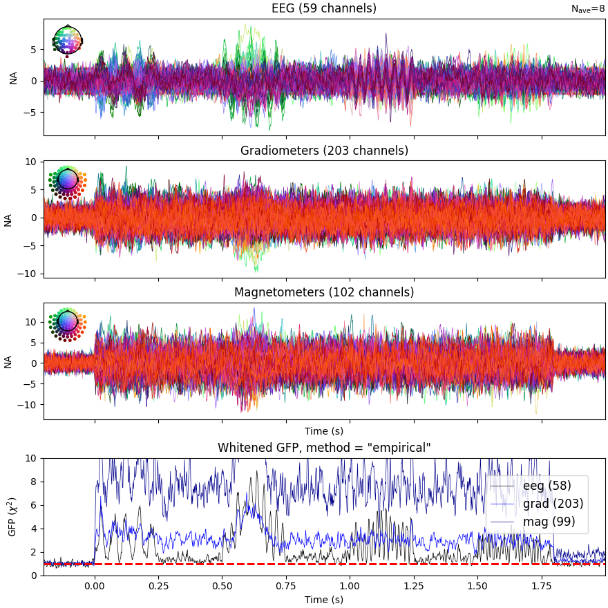
Plot evoked data
events = find_events(raw_sim)  # only 1 pos, so event number == 1
epochs = Epochs(raw_sim, events, 1, tmin=-0.2, tmax=epoch_duration)
cov = compute_covariance(
    epochs, tmax=0.0, method="empirical", verbose="error"
)  # quick calc
evoked = epochs.average()
evoked.plot_white(cov, time_unit="s")

Finding events on: STI 014
Trigger channel STI 014 has a non-zero initial value of 1 (consider using initial_event=True to detect this event)
Removing orphaned offset at the beginning of the file.
9 events found on stim channel STI 014
Event IDs: [1]
Not setting metadata
9 matching events found
Setting baseline interval to [-0.19979521315838786, 0.0] s
Applying baseline correction (mode: mean)
Created an SSP operator (subspace dimension = 4)
4 projection items activated
NOTE: pick_types() is a legacy function. New code should use inst.pick(...).
Computing rank from covariance with rank=None
    Using tolerance 1.2e-14 (2.2e-16 eps * 59 dim * 0.92  max singular value)
    Estimated rank (eeg): 58
    EEG: rank 58 computed from 59 data channels with 1 projector
Computing rank from covariance with rank=None
    Using tolerance 2.1e-13 (2.2e-16 eps * 203 dim * 4.8  max singular value)
    Estimated rank (grad): 203
    GRAD: rank 203 computed from 203 data channels with 0 projectors
Computing rank from covariance with rank=None
    Using tolerance 5.6e-15 (2.2e-16 eps * 102 dim * 0.25  max singular value)
    Estimated rank (mag): 99
    MAG: rank 99 computed from 102 data channels with 3 projectors
    Created an SSP operator (subspace dimension = 4)
Computing rank from covariance with rank={'eeg': 58, 'grad': 203, 'mag': 99, 'meg': 302}
    Setting small MEG eigenvalues to zero (without PCA)
    Setting small EEG eigenvalues to zero (without PCA)
    Created the whitener using a noise covariance matrix with rank 360 (4 small eigenvalues omitted)
Total running time of the script: (0 minutes 12.888 seconds)