mne.read_forward_solution#
- mne.read_forward_solution(fname, include=(), exclude=(), *, ordered=True, verbose=None)[source]#
Read a forward solution a.k.a. lead field.
- Parameters:
- fnamepath-like
The file name, which should end with
-fwd.fif,-fwd.fif.gz,_fwd.fif,_fwd.fif.gz,-fwd.h5, or_fwd.h5.- include
list, optional List of names of channels to include. If empty all channels are included.
- exclude
list, optional List of names of channels to exclude. If empty include all channels.
- orderedbool
If True (default), ensure that the order of the channels in the modified instance matches the order of
ch_names.New in v0.20.0.
Changed in version 1.7: The default changed from False in 1.6 to True in 1.7.
- verbosebool |
str|int|None Control verbosity of the logging output. If
None, use the default verbosity level. See the logging documentation andmne.verbose()for details. Should only be passed as a keyword argument.
- Returns:
- fwdinstance of
Forward The forward solution.
- fwdinstance of
See also
Notes
Forward solutions, which are derived from an original forward solution with free orientation, are always stored on disk as forward solution with free orientation in X/Y/Z RAS coordinates. To apply any transformation to the forward operator (surface orientation, fixed orientation) please apply
convert_forward_solution()after reading the forward solution withread_forward_solution().Forward solutions, which are derived from an original forward solution with fixed orientation, are stored on disk as forward solution with fixed surface-based orientations. Please note that the transformation to surface-based, fixed orientation cannot be reverted after loading the forward solution with
read_forward_solution().
Examples using mne.read_forward_solution#
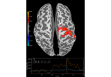
Compute source level time-frequency timecourses using a DICS beamformer
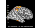
Compute evoked ERS source power using DICS, LCMV beamformer, and dSPM
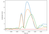
Compute a sparse inverse solution using the Gamma-MAP empirical Bayesian method

Compute sparse inverse solution with mixed norm: MxNE and irMxNE
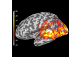
Compute source power estimate by projecting the covariance with MNE
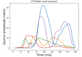
Compute iterative reweighted TF-MxNE with multiscale time-frequency dictionary
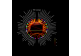
Visualize source leakage among labels using a circular graph
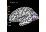
Plot point-spread functions (PSFs) and cross-talk functions (CTFs)
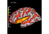
Compute spatial resolution metrics in source space

Compute spatial resolution metrics to compare MEG with EEG+MEG
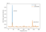
Cortical Signal Suppression (CSS) for removal of cortical signals

Source localization with MNE, dSPM, sLORETA, and eLORETA
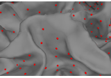
The role of dipole orientations in distributed source localization
Working with CTF data: the Brainstorm auditory dataset
