2.7 Second example of permutation tests

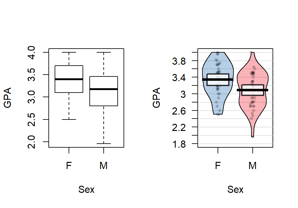
In every chapter, the first example, used to motivate and explain the methods, is followed with a “worked” example where we focus just on the results. In a previous semester, some of the Intermediate Statistics students at Montana State University (n=79) provided information on their Sex³⁹, Age, and current cumulative GPA. We might be interested in whether Males and Females had different average GPAs. First, we can take a look at the difference in the responses by groups based on the output and as displayed in Figure 2.17.

s217 <- read_csv("http://www.math.montana.edu/courses/s217/documents/s217.csv")
library(mosaic)
library(yarrr)

mean(GPA~Sex, data=s217)

##        F        M 
## 3.338378 3.088571

favstats(GPA~Sex, data=s217)

##   Sex  min  Q1 median   Q3 max     mean        sd  n missing
## 1   F 2.50 3.1  3.400 3.70   4 3.338378 0.4074549 37       0
## 2   M 1.96 2.8  3.175 3.46   4 3.088571 0.4151789 42       0

Figure 2.17: Side-by-side boxplot and pirate-plot of GPAs of Intermediate Statistics students by sex.

boxplot(GPA~Sex, data=s217)
pirateplot(GPA~Sex, data=s217, inf.method="ci")

In these data, the distributions of the GPAs look to be left skewed. The Female GPAs look to be slightly higher than for Males (0.25 GPA difference in the means) but is that a “real” difference? We need our inference tools to more fully assess these differences.

First, we can try the parametric approach:

lm_GPA <- lm(GPA~Sex, data=s217)
summary(lm_GPA)

## 
## Call:
## lm(formula = GPA ~ Sex, data = s217)
## 
## Residuals:
##      Min       1Q   Median       3Q      Max 
## -1.12857 -0.28857  0.06162  0.36162  0.91143 
## 
## Coefficients:
##             Estimate Std. Error t value Pr(>|t|)
## (Intercept)  3.33838    0.06766  49.337  < 2e-16
## SexM        -0.24981    0.09280  -2.692  0.00871
## 
## Residual standard error: 0.4116 on 77 degrees of freedom
## Multiple R-squared:  0.08601,    Adjusted R-squared:  0.07414 
## F-statistic: 7.246 on 1 and 77 DF,  p-value: 0.008713

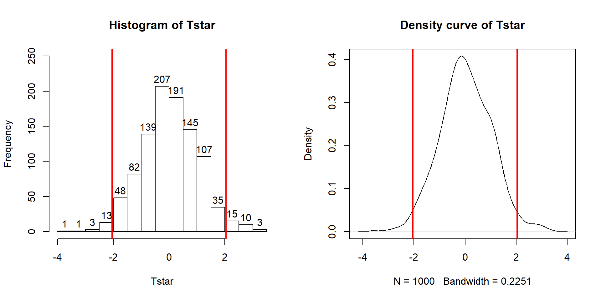
So the test statistic was observed to be \(t=2.69\) and it hopefully follows a \(t(77)\) distribution under the null hypothesis. This provides a p-value of 0.008713 that we can trust if the conditions to use this procedure are at least not clearly violated. Compare these results to the permutation approach, which relaxes that normality assumption, with the results that follow. In the permutation test, \(T=-2.692\) and the p-value is 0.011 which is a little larger than the result provided by the parametric approach. The general agreement of the two approaches, again, provides some re-assurance about the use of either approach when there are not dramatic violations of validity conditions.

B=1000
Tobs <- summary(lm_GPA)$coef[2,3]
Tstar <- matrix(NA, nrow=B)
for (b in (1:B)){
  lmP <- lm(GPA~shuffle(Sex), data=s217)
  Tstar[b] <- summary(lmP)$coef[2,3]
}
pdata(abs(Tstar),abs(Tobs),lower.tail=F)[[1]]

Figure 2.18: Histogram and density curve of permutation distribution of test statistic for Intermediate Statistics student GPAs.

hist(Tstar, labels=T)
abline(v=c(-1,1)*Tobs, lwd=2, col="red")
plot(density(Tstar), main="Density curve of Tstar")
abline(v=c(-1,1)*Tobs, lwd=2, col="red")

Here is a full write-up of the results using all 6+ hypothesis testing steps, using the permutation results for the grade data:

0. The research question involves exploring differences in GPAs between males and females. With data collected from both groups, we should be able to assess this RQ. The pirate-plot with GPAs by gender is a useful visualization. We could use either differences in the sample means or the \(t\)-statistic for the test statistic here.

1. Write the null and alternative hypotheses:

   • \(H_0: \mu_\text{male} = \mu_\text{female}\)

     • where \(\mu_\text{male}\) is the true mean GPA for males and \(\mu_\text{female}\) is true mean GPA for females.

   • \(H_A: \mu_\text{male} \ne \mu_\text{female}\)

2. Plot the data and assess the “Validity Conditions” for the procedure being used:

   • Independent observations condition: It does not appear that this assumption is violated because there is no reason to assume any clustering or grouping of responses that might create dependence in the observations. The only possible consideration is that the observations were taken from different sections and there could be some differences among the sections. However, for overall GPA there is not too much likelihood that the overall GPAs would vary greatly so this not likely to be a big issue. However, it is possible that certain sections (times of day) attract students with different GPA levels.

   • Equal variance condition: There is a small difference in the range of the observations in the two groups but the standard deviations are very similar (close to 0.41) so there is little evidence that this condition is violated.

   • Similar distribution condition: Based on the side-by-side boxplots and pirate-plots, it appears that both groups have slightly left-skewed distributions, which could be problematic for the parametric approach. The two distributions are not exactly alike but they are similar enough that the permutation approach condition is not clearly violated.

3. Find the value of the appropriate test statistic and p-value for your hypotheses:

   • \(T=-2.69\) from the previous R output.

   • p-value=0.011 from the permutation distribution results.

   • This means that there is about a 1.1% chance we would observe a difference in mean GPA (female-male or male-female) of 0.25 points or more if there in fact is no difference in true mean GPA between females and males in Intermediate Statistics in a particular semester.

4. Write a conclusion specific to the problem based on the p-value:

   • There is strong evidence against the null hypothesis of no difference in the true mean GPA between males and females for the Intermediate Statistics students in this semester and so we conclude that there is a difference in the mean GPAs between males and females in these students.

5. Report and discuss an estimate of the size of the differences, with confidence interval(s) if appropriate.

   • Females were estimated to have a higher mean GPA by 0.25 points. The next section discusses confidence intervals that we could add to this result to quantify the uncertainty in this estimate since an estimate without any idea of its precision is only a partial result. This difference of 0.25 on a GPA scale does not seem like a very large difference in the means even though we were able to detect a difference in the groups.

6. Scope of inference:

   • Because this was not a randomized experiment in our explanatory variable, we can’t say that the difference in gender causes the difference in mean GPA. Because it was not a random sample from a larger population (they were asked to participate but not required to and not all the students did participate), our inferences only pertain the Intermediate Statistics students that responded to the survey in that semester.