4.4 Guinea pig tooth growth analysis with Two-Way ANOVA

The effects of dosage and delivery method of ascorbic acid on Guinea Pig odontoblast growth was analyzed as a One-Way ANOVA in Section 3.5 by assessing evidence of any difference in the means of any of the six combinations of dosage method (Vit C capsule vs Orange Juice) and three dosage amounts (0.5, 1, and 2 mg/day). Now we will consider the dosage and delivery methods as two separate variables and explore their potential interaction. A pirate-plot and interaction plot are provided in Figure 2.58.

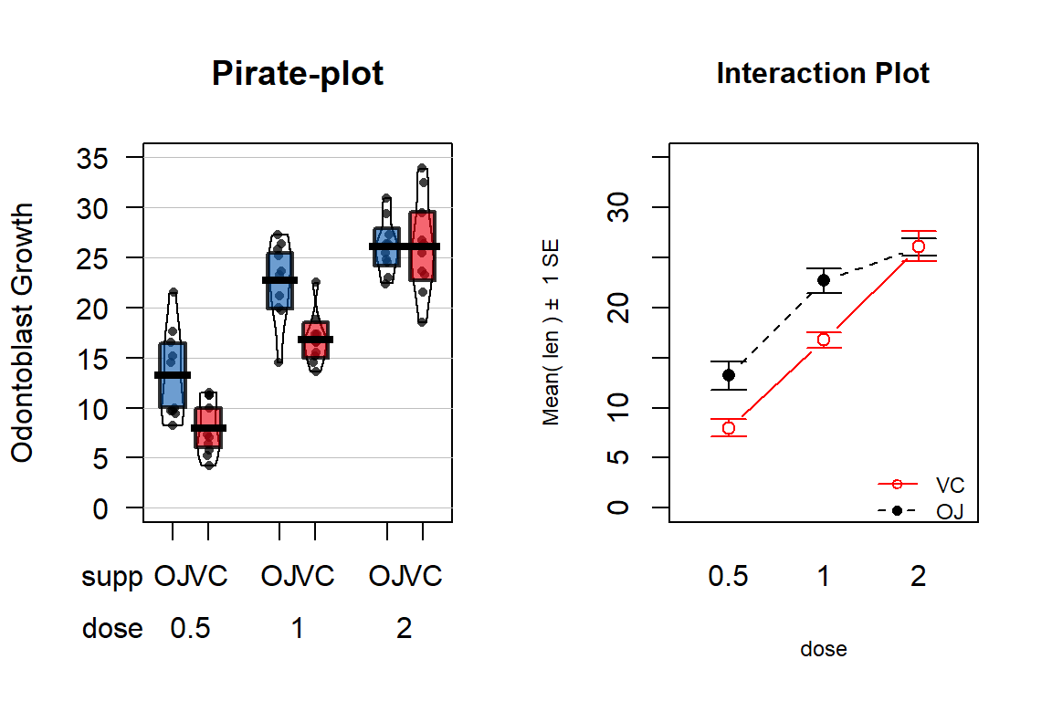
Figure 2.58: Pirate-plot and interaction plot of the odontoblast growth data set.

data(ToothGrowth)
require(tibble)
ToothGrowth <- as_tibble(ToothGrowth)
par(mfrow=c(1,2))
pirateplot(len ~ supp*dose, data=ToothGrowth, ylim=c(0,35),
         main="Pirate-plot",  xlab="Dosage", ylab="Odontoblast Growth", inf.method="ci")
intplot(len~supp*dose, data=ToothGrowth, col=c(1,2), 
        main="Interaction Plot", ylim=c(0,35))

It appears that the effect of method changes based on the dosage as the interaction plot seems to show some evidence of non-parallel lines. Actually, it appears that the effect of delivery method is parallel for doses 0.5 and 1.0 mg/day but that the effect of delivery method changes for 2 mg/day.

We can use the ANOVA \(F\)-test for an interaction to assess whether we think the interaction is “real” relative to the variability in the responses. That is, is it larger than we would expect due to natural variation in the data? If yes, then we think it is a real effect and we should account for it. The following code fits the interaction model and provides an ANOVA table.

TG1 <- lm(len~supp*dose, data=ToothGrowth)
Anova(TG1)

## Anova Table (Type II tests)
## 
## Response: len
##            Sum Sq Df  F value    Pr(>F)
## supp       205.35  1  12.3170 0.0008936
## dose      2224.30  1 133.4151 < 2.2e-16
## supp:dose   88.92  1   5.3335 0.0246314
## Residuals  933.63 56

The R output is reporting an interaction test result of \(F(1,56)=5.3\) with a p-value of 0.025. But this should raise a red flag since the numerator degrees of freedom are not what we should expect based on Table 2.5 of \((K-1)*(J-1) = (2-1)*(3-1)=2\). This brings up an issue in R when working with categorical variables. If the levels of a categorical variable are entered numerically, R will treat them as quantitative variables and not split out the different levels of the categorical variable. To make sure that R treats categorical variables the correct way, we should use the factor function on any variables that are categorical but are coded numerically in the data set. The following code creates a new variable called dosef using the factor function that will help us obtain correct results from the linear model. The re-run of the ANOVA table provides the correct analysis and the expected \(df\) for the two rows of output involving dosef:

ToothGrowth$dosef <- factor(ToothGrowth$dose)
TG2 <- lm(len~supp*dosef, data=ToothGrowth)
Anova(TG2)

## Anova Table (Type II tests)
## 
## Response: len
##             Sum Sq Df F value    Pr(>F)
## supp        205.35  1  15.572 0.0002312
## dosef      2426.43  2  92.000 < 2.2e-16
## supp:dosef  108.32  2   4.107 0.0218603
## Residuals   712.11 54

The ANOVA \(F\)-test for an interaction between supplement type and dosage level is \(F(2,54)= 4.107\) with a p-value of 0.022. So there is moderate to strong evidence against the null hypothesis of no interaction between Dosage and Delivery method, so we would likely conclude that there is an interaction present that we should discuss and this supports a changing effect on odontoblast growth of dosage based on the delivery method in these Guinea Pigs.

Any similarities between this correct result and the previous WRONG result are coincidence. I once attended a Master’s thesis defense where the results from a similar model were not as expected (small p-values in places they didn’t expect and large p-values in places where they thought differences existed based on past results and plots of the data). During the presentation, the student showed some ANOVA tables and the four level categorical variable had 1 numerator \(df\) in all ANOVA tables. The student passed with major revisions but had to re-run all the results and re-write all the conclusions… So be careful to check the ANOVA results (\(df\) and for the right number of expected model coefficients) to make sure they match your expectations. This is one reason why you will be learning to fill in ANOVA tables based on information about the study so that you can be prepared to detect when your code has let you down⁷⁷. It is also a great reason to explore term-plots and coefficient interpretations as that can also help diagnose errors in model construction.

Getting back to the previous results, we now have enough background information to more formally write up a focused interpretation of these results. The 6+ hypothesis testing steps in this situation would be focused on first identifying that the best analysis here is as a Two-Way ANOVA situation (these data were analyzed in Chapter ?? as a One-Way ANOVA but this version is likely better because it can explore whether there is an interaction between delivery method and dosage). We will focus on assessing the interaction. If the interaction had been dropped, we would have reported the test results for the interaction, then re-fit the additive model and used it to explore the main effect tests and estimates for Dose and Delivery method. But since we are inclined to retain the interaction component in the model, the steps focus on the interaction.

0. The RQ is whether there is an interaction of dosage and delivery method on odontoblast growth. Data were collected at all combinations of these predictor variables on the size of the cells, so they can address the size of the cells in these condition combinations. The interaction \(F\)-test will be used to assess the research question.

1. Hypotheses:

   • \(H_0\): No interaction between Delivery method and Dose on odontoblast growth in population of guinea pigs

     \(\Leftrightarrow\) All \(\omega_{jk}\text{'s}=0\).

   • \(H_A\): Interaction between Delivery method and Dose on odontoblast growth in population of guinea pigs

     \(\Leftrightarrow\) At least one \(\omega_{jk}\ne 0\).

2. Plot the data and assess validity conditions:

   • Independence:

     • There is no indication of an issue with this assumption because we don’t know of a reason why the independence of the measurements of odontoblast growth of across the guinea pigs as studied might be violated.

   • Constant variance:

     • To assess this assumption, we can use the pirate-plot in Figure 2.58, the diagnostic plots in Figure 2.59, and by adding the partial residuals to the term-plot⁷⁸ as shown in 2.60.

     • In the Residuals vs Fitted and the Scale-Location plots, the differences in variability among the groups (see the different x-axis positions for each group’s fitted values) is minor, so there is not strong evidence of a problem with the equal variance assumption. Similarly, the original pirate-plots and adding the partial residuals to the term-plot do not highlight big differences in variability at any of the combinations of the predictors, so do not suggest clear issues with this assumption.

     par(mfrow=c(2,2))
     plot(TG2, pch=16) 

     

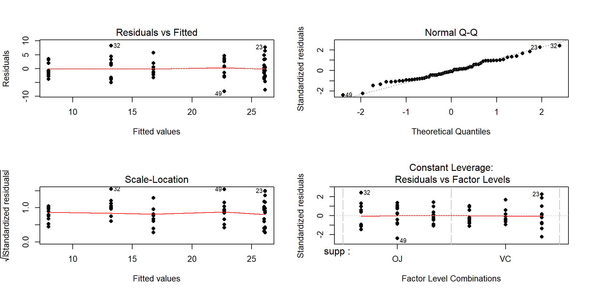
     Figure 2.59: Diagnostic plots for the interaction model for odontoblast growth interaction model.

     plot(allEffects(TG2, residuals = T, x.var="dosef")) 

     

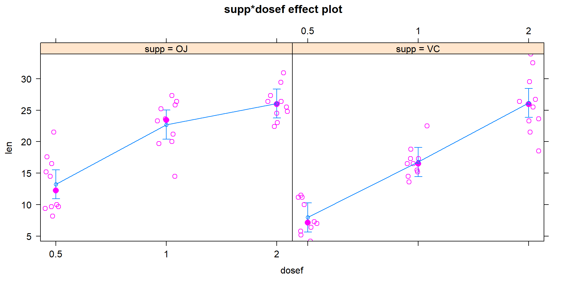
     Figure 2.60: Term-plot for odontoblast growth interaction model with partial residuals added.

   • Normality of residuals:

     • The QQ-Plot in Figure 2.59 does not suggest a problem with this assumption.

Note that these diagnostics and conclusions are the same as in Section 3.5 because the interaction model and the One-Way ANOVA model with all six combinations of the levels of the two variables fit exactly the same. But the RQ that we can address differs due to the different model parameterizations.

3. Calculate the test statistic and p-value for the interaction test.

   TG2 <- lm(len~supp*dosef, data=ToothGrowth)
   Anova(TG2) 

   ## Anova Table (Type II tests)
   ## 
   ## Response: len
   ##             Sum Sq Df F value    Pr(>F)
   ## supp        205.35  1  15.572 0.0002312
   ## dosef      2426.43  2  92.000 < 2.2e-16
   ## supp:dosef  108.32  2   4.107 0.0218603
   ## Residuals   712.11 54

   • The test statistic is \(F(2,54)=4.107\) with a p-value of 0.0219

   • To find this p-value directly in R from the test statistic value and \(F\)-distribution, we can use the pf function.

   pf(4.107, df1=2, df2=54, lower.tail=F)

   ## [1] 0.0218601

4. Conclusion based on p-value:

   • With a p-value of 0.0219, there is about a 2.19% chance we would observe an interaction like we did (or more extreme) if none were truly present. This provides moderate to strong evidence against the null hypothesis of no interaction between delivery method and dosage on odontoblast growth so we would retain the interaction in the model.

5. Size of differences:

   • See discussion below.

6. Scope of Inference:

   • Based on the random assignment of treatment levels, causal inference is possible but because the guinea pigs were not randomly selected, the inferences only pertain to these guinea pigs.

In a Two-Way ANOVA, we need to go a little further to get to the final “size” interpretations since the models are more complicated. When there is an interaction present, we should focus on the term-plot of the interaction model for an interpretation of the form and pattern of the interaction. If the interaction were unimportant, then the hypotheses and results should focus on the additive model results, especially the estimated model coefficients. To see why we don’t usually discuss all the estimated model coefficients in an interaction model, the six coefficients for this model are provided:

summary(TG2)$coefficients

##               Estimate Std. Error    t value     Pr(>|t|)
## (Intercept)      13.23   1.148353 11.5208468 3.602548e-16
## suppVC           -5.25   1.624017 -3.2327258 2.092470e-03
## dosef1            9.47   1.624017  5.8312215 3.175641e-07
## dosef2           12.83   1.624017  7.9001660 1.429712e-10
## suppVC:dosef1    -0.68   2.296706 -0.2960762 7.683076e-01
## suppVC:dosef2     5.33   2.296706  2.3207148 2.410826e-02

There are two \(\hat{\omega}_{jk}\text{'s}\) in the results, related to modifying the estimates for doses of 1 (-0.68) and 2 (5.33) for the Vitamin C group. If you want to re-construct the fitted values from the model that are displayed in Figure 2.61, you have to look for any coefficients that are “turned on” for a combination of levels of interest. For example, for the OJ group (solid line), the dosage of 0.5 mg/day has an estimate of an average growth of approximately 13 mm. This is the baseline group, so the model estimate for an observation in the OJ and 0.5 mg/day dosage is simply \(\hat{y}_{i,\text{OJ},0.5mg}=\hat{\alpha}=13.23\) microns. For the OJ and 2 mg/day dosage estimate that has a value over 25 microns in the plot, the model incorporates the deviation for the 2 mg/day dosage: \(\hat{y}_{i,\text{OJ},2mg}=\hat{\alpha} + \hat{\tau}_{2mg}=13.23 + 12.83 = 26.06\) microns. For the Vitamin C group, another coefficient becomes involved from its “main effect”. For the VC and 0.5 mg dosage level, the estimate is approximately 8 microns. The pertinent model components are \(\hat{y}_{i,\text{VC},0.5mg}=\hat{\alpha} + \hat{\gamma}_{\text{VC}}=13.23 + (-5.25) = 7.98\) microns. Finally, when we consider non-baseline results for both groups, three coefficients are required to reconstruct the results in the plot. For example, the estimate for the VC, 1 mg dosage is \(\hat{y}_{i,\text{VC},1mg}=\hat{\alpha} + \hat{\tau}_{1mg} + \hat{\gamma}_{\text{VC}} + \hat{\omega}_{\text{VC},1mg} = 13.23 + 9.47 + (-5.25) +(-0.68)= 16.77\) microns. We usually will by-pass all this fun(!) with the coefficients in an interaction model and go from the ANOVA interaction test to focusing on the pattern of the responses in the interaction plot or going to the simpler additive model, but it is good to know that there are still model coefficients driving our results even if there are too many to be easily interpreted.

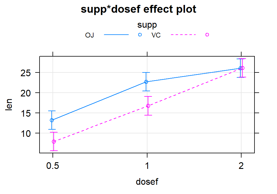
Figure 2.61: Term-plot for the estimated interaction for the Odontoblast Growth data using the multiline=T and ci.style="bars" options.

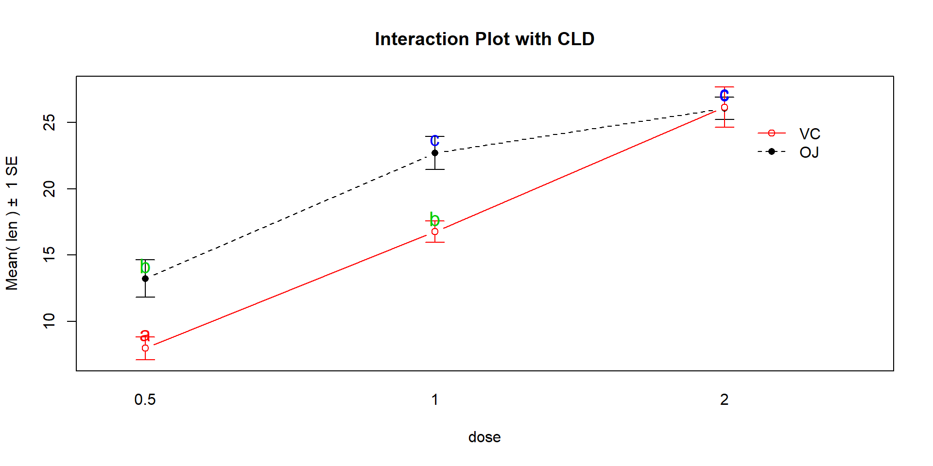
Figure 2.62: Interaction plot for Odontoblast data with added CLD from Tukey’s HSD.

plot(allEffects(TG2), grid=T, multiline=T, lty=c(1,2), ci.style="bars")

Given the presence of an important interaction, then the final step in the interpretation here is to interpret the results in the interaction plot or term-plot of the interaction model, supported by the p-value suggesting a different effect of supplement type based on the dosage level. To supplement this even more, knowing which combinations of levels differ can enhance our discussion. Tukey’s HSD results (specifically the CLD) can be added to the original interaction plot by turning on the cld=T option in the intplot function as seen in Figure 2.62. Sometimes it is hard to see the letters and so there is also a cldshift=... option to move the letters up or down; here a value of 1 seemed to work.

intplot(len~supp*dose, data=ToothGrowth, col=c(1,2), cldshift=1,
        cld=T, main="Interaction Plot with CLD")

The “size” interpretation of the previous hypothesis test result could be something like the following: Generally increasing the dosage increases the mean growth except for the 2 mg/day dosage level where the increase levels off in the OJ group (OJ 1 and 2 mg/day are not detectably different) and the differences between the two delivery methods disappear at the highest dosage level. But for 0.5 and 1 mg/day dosages, OJ is clearly better than VC by about 10 microns of growth on average.