8.3 Interpretation of MLR terms

Since these results (finally) do not contain any highly influential points, we can formally discuss interpretations of the slope coefficients and how the term-plots (Figure 2.158) aid our interpretations. Term-plots in MLR are constructed by holding all the other quantitative variables¹¹⁹ at their mean and generating predictions and 95% CIs for the mean response across the levels of observed values for each predictor variable. This idea also helps us to work towards interpretations of each term in an MLR model. For example, for Elevation, the term-plot starts at an elevation around 5000 feet and ends at an elevation around 8000 feet. To generate that line and CIs for the mean snow depth at different elevations, the MLR model of

\[\widehat{\text{SnowDepth}}_i = -213.3 + 0.0269\cdot\text{Elevation}_i +0.984\cdot\text{MinTemp}_i +1.243\cdot\text{MaxTemp}_i\]

is used, but we need to have “something” to put in for the two temperature variables to predict Snow Depth for different Elevations. The typical convention is to hold the “other” variables at their means to generate these plots. This tactic also provides a way of interpreting each slope coefficient. Specifically, we can interpret the Elevation slope as: For a 1 foot increase in Elevation, we estimate the mean Snow Depth to increase by 0.0269 inches, holding the minimum and maximum temperatures constant. More generally, the slope interpretation in an MLR is:

For a 1 [units of \(\boldsymbol{x_k}\)] increase in \(\boldsymbol{x_k}\), we estimate the mean of \(\boldsymbol{y}\) to change by \(\boldsymbol{b_k}\) [units of y], after controlling for [list of other explanatory variables in model].

To make this more concrete, we can recreate some points in the Elevation term-plot. To do this, we first need the mean of the “other” predictors, Min.Temp and Max.Temp.

mean(snotel2[-c(9,22),]$Min.Temp)

## [1] 27.82609

mean(snotel2[-c(9,22),]$Max.Temp)

## [1] 36.3913

We can put these values into the MLR equation and simplify it by combining like terms, to an equation that is in terms of just Elevation given that we are holding Min.Temp and Max.Temp at their means:

\[\begin{array}{rl} \widehat{\text{SnowDepth}}_i &= -213.3 + 0.0269\cdot\text{Elevation}_i +0.984*\boldsymbol{27.826} +1.243*\boldsymbol{36.391} \\ &= -213.3 + 0.0269\cdot\text{Elevation}_i + 27.38 + 45.23 \\ &= \boldsymbol{-140.69 + 0.0269\cdot\textbf{Elevation}_i}. \end{array}\]

So at the means on the two temperature variables, the model looks like an SLR with an estimated y-intercept of -140.69 (mean Snow Depth for Elevation of 0 if temperatures are at their means) and an estimated slope of 0.0269. Then we can plot the predicted changes in \(y\) across all the values of the predictor variable (Elevation) while holding the other variables constant. To generate the needed values to define a line, we can plug various Elevation values into the simplified equation:

• For an elevation of 5000 at the average temperatures, we predict a mean snow depth of \(-140.69 + 0.0269*5000 = -6.19\) inches.

• For an elevation of 6000 at the average temperatures, we predict a mean snow depth of \(-140.69 + 0.0269*6000 = 20.71\) inches.

• For an elevation of 8000 at the average temperatures, we predict a mean snow depth of \(-140.69 + 0.0269*8000 = 74.51\) inches.

We can plot this information (Figure 2.160) using the plot function to show the points we calculated and the lines function to add a line that connects the dots. In the plot function, we used the ylim=... option to make the scaling on the y-axis match the previous term-plot’s scaling.

(ref:fig8-10) Term-plot for Elevation “by-hand”, holding temperature variables constant at their means.

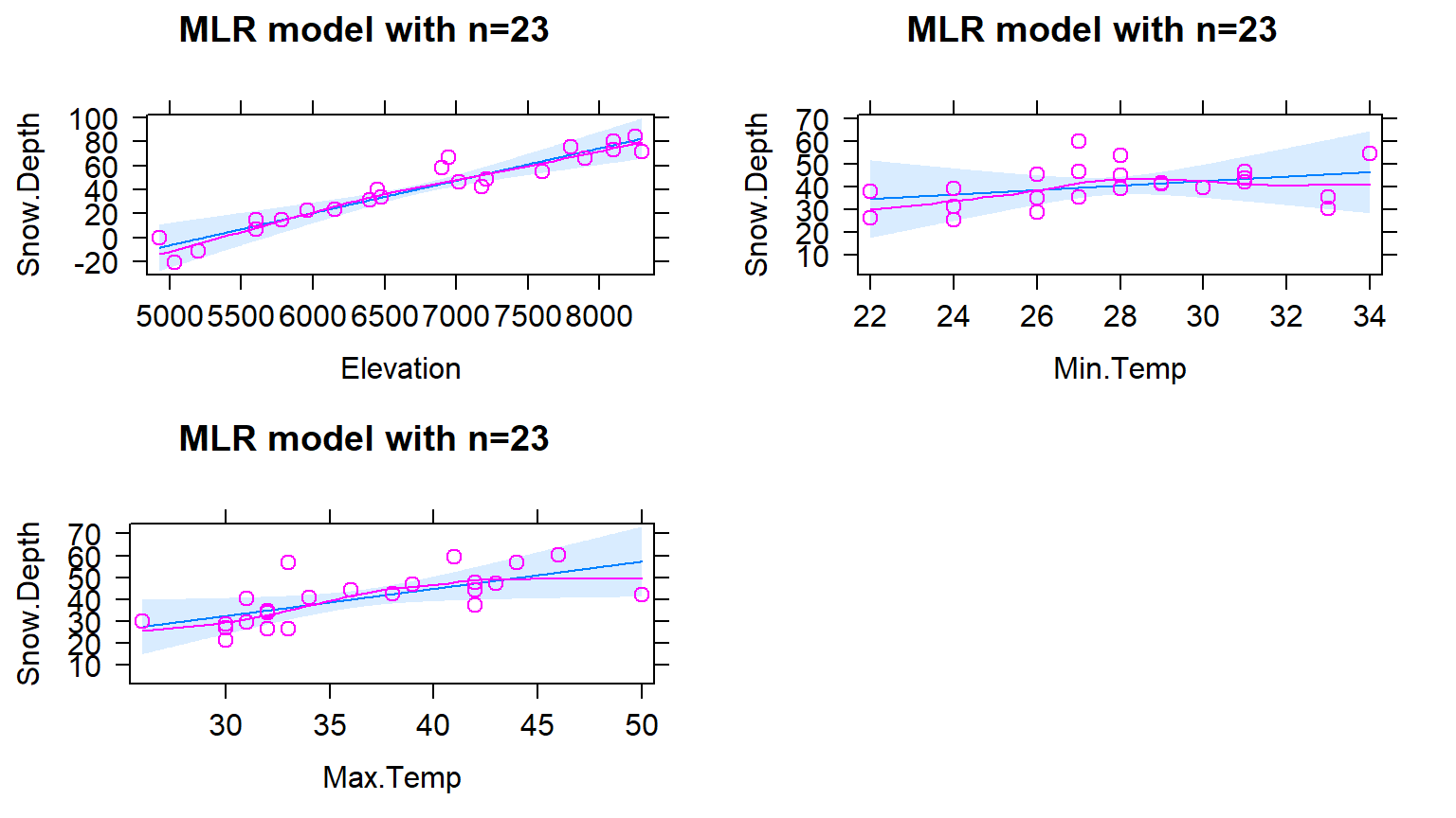
Figure 2.160: (ref:fig8-10)

#Making own effect plot:
elevs <- c(5000,6000,8000)
snowdepths <- c(-6.19,20.71,74.51)
plot(snowdepths~elevs, ylim=c(-20,90), cex=2, col="blue", pch=16,
     main="Effect plot of elevation by hand")
lines(snowdepths~elevs, col="red", lwd=2)

Note that we only needed 2 points to define the line but need a denser grid of elevations if we want to add the 95% CIs for the true mean snow depth across the different elevations since they vary as a function of the distance from the mean of the explanatory variables.

To get the associated 95% CIs, we could return to using the predict function for the MLR, again holding the temperatures at their mean values. The predict function is sensitive and needs the same variable names as used in the original model fitting to work. First we create a “new” data set using the seq function to generate the desired grid of elevations and the rep function¹²⁰ to repeat the means of the temperatures for each of elevation values we need to make the plot. The code creates a specific version of the predictor variables to force the predict function to provide fitted values and CIs across different elevations with temperatures held constant that is stored in newdata1.

elevs <- seq(from=5000, to=8000, length.out=30)
newdata1 <- tibble(Elevation=elevs, Min.Temp=rep(27.826,30),
                       Max.Temp=rep(36.3913,30))
newdata1

## # A tibble: 30 x 3
##    Elevation Min.Temp Max.Temp
##        <dbl>    <dbl>    <dbl>
##  1     5000      27.8     36.4
##  2     5103.     27.8     36.4
##  3     5207.     27.8     36.4
##  4     5310.     27.8     36.4
##  5     5414.     27.8     36.4
##  6     5517.     27.8     36.4
##  7     5621.     27.8     36.4
##  8     5724.     27.8     36.4
##  9     5828.     27.8     36.4
## 10     5931.     27.8     36.4
## # ... with 20 more rows

The predicted snow depths along with 95% confidence intervals for the mean, holding temperatures at their means, are:

predict(m6, newdata=newdata1, interval="confidence")

##           fit        lwr      upr
## 1  -6.3680312 -24.913607 12.17754
## 2  -3.5898846 -21.078518 13.89875
## 3  -0.8117379 -17.246692 15.62322
## 4   1.9664088 -13.418801 17.35162
## 5   4.7445555  -9.595708 19.08482
## 6   7.5227022  -5.778543 20.82395
## 7  10.3008489  -1.968814 22.57051
## 8  13.0789956   1.831433 24.32656
## 9  15.8571423   5.619359 26.09493
## 10 18.6352890   9.390924 27.87965
## 11 21.4134357  13.140233 29.68664
## 12 24.1915824  16.858439 31.52473
## 13 26.9697291  20.531902 33.40756
## 14 29.7478758  24.139153 35.35660
## 15 32.5260225  27.646326 37.40572
## 16 35.3041692  31.002236 39.60610
## 17 38.0823159  34.139812 42.02482
## 18 40.8604626  36.997617 44.72331
## 19 43.6386092  39.559231 47.71799
## 20 46.4167559  41.866745 50.96677
## 21 49.1949026  43.988619 54.40119
## 22 51.9730493  45.985587 57.96051
## 23 54.7511960  47.900244 61.60215
## 24 57.5293427  49.759987 65.29870
## 25 60.3074894  51.582137 69.03284
## 26 63.0856361  53.377796 72.79348
## 27 65.8637828  55.154251 76.57331
## 28 68.6419295  56.916422 80.36744
## 29 71.4200762  58.667725 84.17243
## 30 74.1982229  60.410585 87.98586

So we could do this with any model for each predictor variable to create term-plots, or we can just use the allEffects function to do this for us. This exercise is useful to complete once to understand what is being displayed in term-plots but using the allEffects function makes getting these plots much easier.

There are two other model components of possible interest in this model. The slope of 0.984 for Min.Temp suggests that for a 1\(^\circ F\) increase in Minimum Temperature, we estimate a 0.984 inch change in the mean Snow Depth, after controlling for Elevation and Max.Temp at the sites. Similarly, the slope of 1.243 for the Max.Temp suggests that for a 1\(^\circ F\) increase in Maximum Temperature, we estimate a 1.243 inch change in the mean Snow Depth, holding Elevation and Min.Temp constant. Note that there are a variety of ways to note that each term in an MLR is only a particular value given the other variables in the model. We can use words such as “holding the other variables constant” or “after adjusting for the other variables” or “in a model with…” or “for observations with similar values of the other variables but a difference of 1 unit in the predictor..”. The main point is to find words that reflect that this single slope coefficient might be different if we had a different overall model and the only way to interpret it is conditional on the other model components.

Term-plots have a few general uses to enhance our regular slope interpretations. They can help us assess how much change in the mean of \(y\) the model predicts over the range of each observed \(x\). This can help you to get a sense of the “practical” importance of each term. Additionally, the term-plots show 95% confidence intervals for the mean response across the range of each variable, holding the other variables at their means. These intervals can be useful for assessing the precision in the estimated mean at different values of each predictor. However, note that you should not use these plots for deciding whether the term should be retained in the model – we have other tools for making that assessment. And one last note about term-plots – they do not mean that the relationships are really linear between the predictor and response variable being displayed. The model forces the relationship to be linear even if that is not the real functional form. Term-plots are not diagnostics for the model unless you add the partial residuals, the lines are just summaries of the model you assumed was correct! Any time we do linear regression, the inferences are contingent upon the model we chose. We know our model is not perfect, but we hope that it helps us learn something about our research question(s) and, to trust its results, we hope it matches the data fairly well.