6.6 Describing relationships with a regression model

When the relationship appears to be relatively linear, it makes sense to estimate and then interpret a line to represent the relationship between the variables. This line is called a regression line and involves finding a line that best fits (explains variation in) the response variable for the given values of the explanatory variable. For regression, it matters which variable you choose for \(x\) and which you choose for \(y\) – for correlation it did not matter. This regression line describes the “effect” of \(x\) on \(y\) and also provides an equation for predicting values of \(y\) for given values of \(x\). The Beers and BAC data provide a nice example to start our exploration of regression models. The beer consumption is a clear explanatory variable, detectable in the story because (1) it was randomly assigned to subjects and (2) basic science supports beer consumption amount being an explanatory variable for BAC. In some situations, this will not be so clear, but look for random assignment or scientific logic to guide your choices of variables as explanatory or response⁹⁸. Regression lines are actually provided by default in the scatterplot function with the reg.line=T option or just omitting reg.line=F from the previous versions of the code since it is a default option to provide the lines.

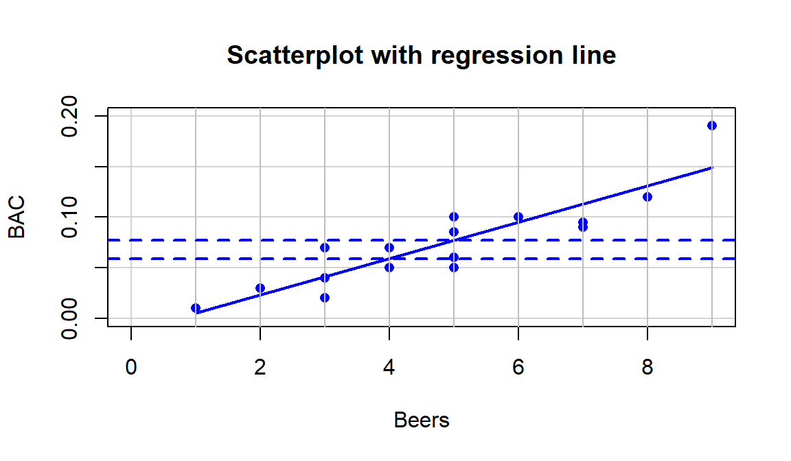
(ref:fig6-13) Scatterplot with estimated regression line for the Beers and BAC data. Horizontal dashed lines for the predicted BAC for 4 and 5 beers consumed.

scatterplot(BAC~Beers, ylim=c(0,.2), xlim=c(0,9), data=BB,
            boxplot=F, main="Scatterplot with regression line",
            lwd=2, smooth=F)
abline(v=1:9, col="grey")
abline(h=c(0.05914,0.0771), col="blue", lty=2, lwd=2)

Figure 2.112: (ref:fig6-13)

The equation for a line is \(y=a+bx\), or maybe \(y=mx+b\). In the version \(mx+b\) you learned that \(m\) is a slope coefficient that relates a change in \(x\) to changes in \(y\) and that \(b\) is a y-intercept (the value of \(y\) when \(x\) is 0). In Figure 2.112, two extra horizontal lines are added to help you see the defining characteristics of the line. The slope, whatever letter you use, is the change in \(y\) for a one-unit increase in \(x\). Here, the slope is the change in BAC for a 1 beer increase in Beers, such as the change from 4 to 5 beers. The y-values (blue, dashed lines) for Beers = 4 and 5 go from 0.059 to 0.077. This means that for a 1 beer increase (+1 unit change in \(x\)), the BAC goes up by \(0.077-0.059=0.018\) (+0.018 unit change in \(y\)). We can also try to find the y-intercept on the graph by looking for the BAC level for 0 Beers consumed. The y-value (BAC) ends up being around -0.01 if you extend the regression line to Beers=0. You might assume that the BAC should be 0 for Beers=0 but the researchers did not observe any students at 0 Beers, so we don’t really know what the BAC might be at this value. We have to use our line to predict this value. This ends up providing a prediction below 0 – an impossible value for BAC. If the y-intercept were positive, it would suggest that the students has a BAC over 0 even without drinking.

The numbers reported were very accurate because we weren’t using the plot alone to generate the values – we were using a linear model to estimate the equation to describe the relationship between Beers and BAC. In statistics, we estimate “\(m\)” and “\(b\)”. We also write the equation starting with the y-intercept and use slightly different notation that allows us to extend to more complicated models with more variables. Specifically, the estimated regression equation is \(\hat{y} = b_0 + b_1x\), where

• \(\hat{y}\) is the estimated value of \(y\) for a given \(x\),

• \(b_0\) is the estimated y-intercept (predicted value of \(y\) when \(x\) is 0),

• \(b_1\) is the estimated slope coefficient, and

• \(x\) is the explanatory variable.

One of the differences between when you learned equations in algebra classes and our situation is that the line is not a perfect description of the relationship between \(x\) and \(y\) – it is an “on average” description and will usually leave differences between the line and the observations, which we call residuals \((e = y-\hat{y})\). We worked with residuals in the ANOVA⁹⁹ material. The residuals describe the vertical distance in the scatterplot between our model (regression line) and the actual observed data point. The lack of a perfect fit of the line to the observations distinguishes statistical equations from those you learned in math classes. The equations work the same, but we have to modify interpretations of the coefficients to reflect this.

We also tie this estimated model to a theoretical or population regression model:

\[y_i = \beta_0 + \beta_1x_i+\varepsilon_i\]

where:

• \(y_i\) is the observed response for the \(i^{th}\) observation,

• \(x_i\) is the observed value of the explanatory variable for the \(i^{th}\) observation,

• \(\beta_0 + \beta_1x_i\) is the true mean function evaluated at \(x_i\),

• \(\beta_0\) is the true (or population) y-intercept,

• \(\beta_1\) is the true (or population) slope coefficient, and

• the deviations, \(\varepsilon_i\), are assumed to be independent and normally distributed with mean 0 and standard deviation \(\sigma\) or, more compactly, \(\varepsilon_i \sim N(0,\sigma^2)\).

This presents another version of the linear model from Chapters 2, ??, and ??, now with a quantitative explanatory variable instead of categorical explanatory variable(s). This chapter focuses mostly on the estimated regression coefficients, but remember that we are doing statistics and our desire is to make inferences to a larger population. So, estimated coefficients, \(b_0\) and \(b_1\), are approximations to theoretical coefficients, \(\beta_0\) and \(\beta_1\). In other words, \(b_0\) and \(b_1\) are the statistics that try to estimate the true population parameters \(\beta_0\) and \(\beta_1\), respectively.

To get estimated regression coefficients, we use the lm function and our standard lm(y~x, data=...) setup. This is the same function used to estimate our ANOVA models and much of this will look familiar. In fact, the ties between ANOVA and regression are deep and fundamental but not the topic of this section. For the Beers and BAC example, the estimated regression coefficients can be found from:

m1 <- lm(BAC~Beers, data=BB)
m1

## 
## Call:
## lm(formula = BAC ~ Beers, data = BB)
## 
## Coefficients:
## (Intercept)        Beers  
##    -0.01270      0.01796

More often, we will extract these from the coefficient table produced by a model summary:

summary(m1)

## 
## Call:
## lm(formula = BAC ~ Beers, data = BB)
## 
## Residuals:
##       Min        1Q    Median        3Q       Max 
## -0.027118 -0.017350  0.001773  0.008623  0.041027 
## 
## Coefficients:
##              Estimate Std. Error t value Pr(>|t|)
## (Intercept) -0.012701   0.012638  -1.005    0.332
## Beers        0.017964   0.002402   7.480 2.97e-06
## 
## Residual standard error: 0.02044 on 14 degrees of freedom
## Multiple R-squared:  0.7998, Adjusted R-squared:  0.7855 
## F-statistic: 55.94 on 1 and 14 DF,  p-value: 2.969e-06

From either version of the output, you can find the estimated y-intercept in the (Intercept) part of the output and the slope coefficient in the Beers part of the output. So \(b_0 = -0.0127\), \(b_1=0.01796\), and the estimated regression equation is

\[\widehat{\text{BAC}}_i = -0.0127 + 0.01796\cdot\text{Beers}_i.\]

This is the equation that was plotted in Figure 2.112. In writing out the equation, it is good to replace \(x\) and \(y\) with the variable names to make the predictor and response variables clear. If you prefer to write all equations with \(\boldsymbol{x}\) and \(\boldsymbol{y}\), you need to define \(\boldsymbol{x}\) and \(\boldsymbol{y}\) or else these equations are not clearly defined.

There is a general interpretation for the slope coefficient that you will need to master. In general, we interpret the slope coefficient as:

• Slope interpretation (general): For a 1 [unit of X] increase in X, we expect, on average, a \(\boldsymbol{b_1}\) [unit of Y] change in Y.

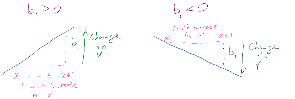
Figure 2.113 can help you think about the different sorts of slope coefficients we might need to interpret, both providing changes in the response variable for 1 unit increases in the predictor variable.

Figure 2.113: Diagram of interpretation of slope coefficients.

Applied to this problem, for each additional 1 beer consumed, we expect a 0.018 gram per dL change in the BAC on average. Using “change” in the interpretation for what happened in the response allows you to use the same template for the interpretation even with negative slopes – be careful about saying “decrease” when the slope is negative as you can create a double-negative and end up implying an increase… Note also that you need to carefully incorporate the units of \(x\) and the units of \(y\) to make the interpretation clear. For example, if the change in BAC for 1 beer increase is 0.018, then we could also modify the size of the change in \(x\) to be a 10 beer increase and then the estimated change in BAC is \(10*0.018 = 0.18\) g/dL. Both are correct as long as you are clear about the change in \(x\) you are talking about. Typically, we will just use the units used in the original variables and only change the scale of “change in \(x\)” when it provides an interpretation we are particularly interested in.

Similarly, the general interpretation for a y-intercept is:

• Y-intercept interpretation (general): For X= 0 [units of X], we expect, on average, \(\boldsymbol{b_0}\) [units of Y] in Y.

Again, applied to the BAC data set: For 0 beers for Beers consumed, we expect, on average, -0.012 g/dL BAC. The y-intercept interpretation is often less interesting than the slope interpretation but can be interesting in some situations. Here, it is predicting average BAC for Beers=0, which is a value outside the scope of the \(x\text{'s}\) (Beers was observed between 1 and 9). Prediction outside the scope of the predictor values is called extrapolation. Extrapolation is dangerous at best and misleading at worst. That said, if you are asked to interpret the y-intercept you should still interpret it, but it is also good to note if it is outside of the region where we had observations on the explanatory variable. Another example is useful for practicing how to do these interpretations.

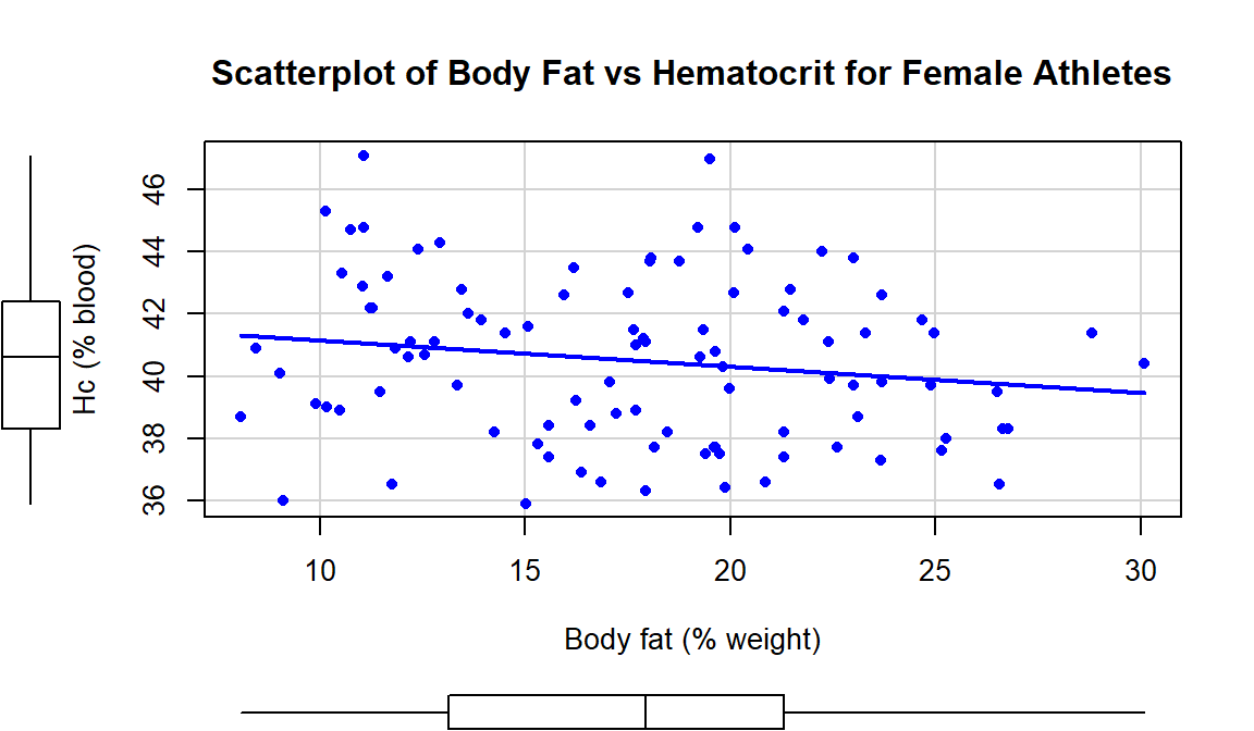
In the Australian Athlete data, we saw a weak negative relationship between Body Fat (% body weight that is fat) and Hematocrit (% red blood cells in the blood). The scatterplot in Figure 2.114 shows just the results for the female athletes along with the regression line which has a negative slope coefficient. The estimated regression coefficients are found using the lm function:

aisR2 <- ais[-c(56,166), c("Ht","Hc","Bfat","Sex")]
m2 <- lm(Hc~Bfat, data=subset(aisR2,Sex==1)) #Results for Females 

summary(m2)

## 
## Call:
## lm(formula = Hc ~ Bfat, data = subset(aisR2, Sex == 1))
## 
## Residuals:
##     Min      1Q  Median      3Q     Max 
## -5.2399 -2.2132 -0.1061  1.8917  6.6453 
## 
## Coefficients:
##             Estimate Std. Error t value Pr(>|t|)
## (Intercept) 42.01378    0.93269  45.046   <2e-16
## Bfat        -0.08504    0.05067  -1.678   0.0965
## 
## Residual standard error: 2.598 on 97 degrees of freedom
## Multiple R-squared:  0.02822,    Adjusted R-squared:  0.0182 
## F-statistic: 2.816 on 1 and 97 DF,  p-value: 0.09653

scatterplot(Hc~Bfat, data=subset(aisR2,Sex==1), smooth=F,
            main="Scatterplot of Body Fat vs Hematocrit for Female Athletes",
            ylab="Hc (% blood)", xlab="Body fat (% weight)")

Figure 2.114: Scatterplot of Hematocrit versus Body Fat for female athletes.

Based on these results, the estimated regression equation is \(\widehat{\text{Hc}}_i = 42.014 - 0.085\cdot\text{BodyFat}_i\) with \(b_0 = 42.014\) and \(b_1 = 0.085\). The slope coefficient interpretation is: For a one percent increase in body fat, we expect, on average, a -0.085% (blood) change in Hematocrit for Australian female athletes. For the y-intercept, the interpretation is: For a 0% body fat female athlete, we expect a Hematocrit of 42.014% on average. Again, this y-intercept involves extrapolation to a region of \(x\)’s that we did not observed. None of the athletes had body fat below 5% so we don’t know what would happen to the hematocrit of an athlete that had no body fat except that it probably would not continue to follow a linear relationship.