5.6 Chi-square distribution for the \(X^2\) statistic

When one additional assumption beyond the previous assumptions for the permutation test is met, it is possible to avoid permutations to find the distribution of the \(X^2\) statistic under the null hypothesis and get a p-value using what is called the Chi-square or \(\boldsymbol{\chi^2}\)-distribution. The name of our test statistic, X-squared, is meant to allude to the potential that this will follow a \(\boldsymbol{\chi^2}\)-distribution in certain situations but may not do that all the time and we still can use the methods in Section 5.5. Along with the previous assumption regarding independence and all expected cell counts are greater than 0, we make a requirement that N (the total sample size) is “large enough” and this assumption is written in terms of the expected cell counts. If N is large, then all the expected cell counts should also be large because all those observations have to go somewhere. The problems for the \(\boldsymbol{\chi^2}\)-distribution as an approximation to the distribution of the \(X^2\) statistic under the null hypothesis come when expected cell counts are below 5. And the smaller the expected cell counts become, the more problematic the \(\boldsymbol{\chi^2}\)-distribution is as an approximation of the sampling distribution of the \(X^2\) statistic under the null hypothesis. The standard rule of thumb is that all the expected cell counts need to exceed 5 for the parametric approach to be valid. When this condition is violated, it is better to use the permutation approach. The chisq.test function will provide a warning message to help you notice this. But it is good practice to always explore the expected cell counts using chisq.test(...)$expected.

chisq.test(Arthtable)$expected

##          Improved
## Treatment None     Some   Marked
##   Placebo 21.5 7.166667 14.33333
##   Treated 20.5 6.833333 13.66667

In the Arthritis data set, the sample size was sufficiently large for the \(\boldsymbol{\chi^2}\)-distribution to provide an accurate p-value since the smallest expected cell count is 6.833 (so all expected counts are larger than 5).

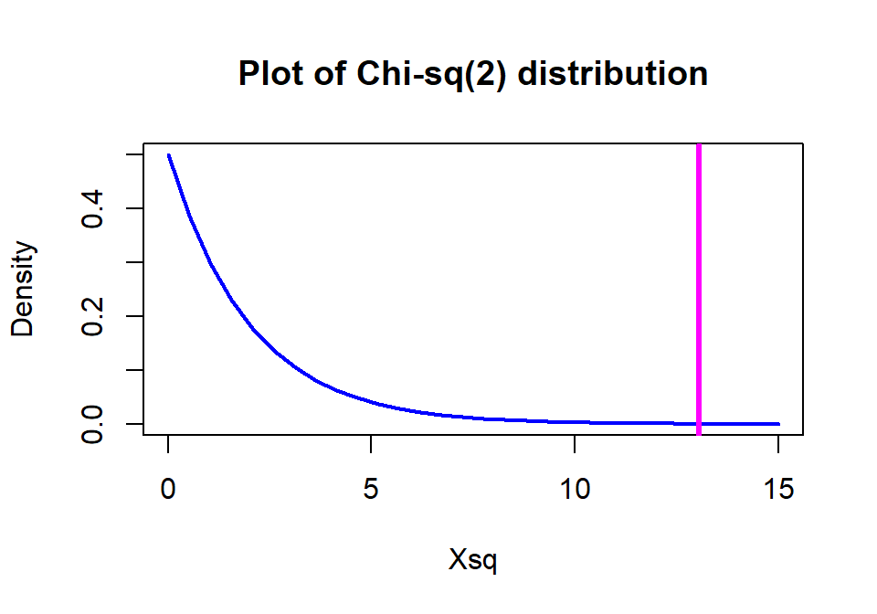
The \(\boldsymbol{\chi^2}\)-distribution is a right-skewed distribution that starts at 0 as shown in Figure 2.81. Its shape changes as a function of its degrees of freedom. In the contingency table analyses, the degrees of freedom for the Chi-square test are calculated as

\[\textbf{DF} \mathbf{=(R-1)*(C-1)} = (\text{number of rows }-1)* (\text{number of columns }-1).\]

In the \(2 \times 3\) table above, the \(\text{DF}=(2-1)*(3-1)=2\) leading to a Chi-square distribution with 2 df for the distribution of \(X^2\) under the null hypothesis. The p-value is based on the area to the right of the observed \(X^2\) value of 13.055 and the pchisq function provides that area as 0.00146. Note that this is very similar to the permutation result found previously for these data.

pchisq(13.055, df=2, lower.tail=F)

## [1] 0.001462658

We’ll see more examples of the \(\boldsymbol{\chi^2}\)-distributions in each of the examples that follow.

(ref:fig5-10) \(\boldsymbol{\chi^2}\)-distribution with two degrees of freedom with the observed statistic of 13.1 indicated with a vertical line.

Figure 2.81: (ref:fig5-10)

A small side note about sample sizes is warranted here. In contingency tables, especially those based on survey data, it is common to have large overall sample sizes (\(N\)). With large sample sizes, it becomes easy to find strong evidence against the null hypothesis, even when the “distance” from the null is relatively minor and possibly unimportant. By this we mean that the observed proportions are a small practical distance from the situation described in the null. After obtaining a small p-value, we need to consider whether we have obtained practical significance (or maybe better described as practical importance) to accompany our discussion of strong evidence against the null hypothesis. Whether a result is large enough to be of practical importance can only be judged by knowing something about the situation we are studying and by providing a good summary of our results to allow experts to assess the size and importance of the result. Unfortunately, many researchers are so happy to see small p-values that this is their last step. We encountered a similar situation in the car overtake distance data set where a large sample size provided a data set that had a small p-value and possibly minor differences in the means driving it.

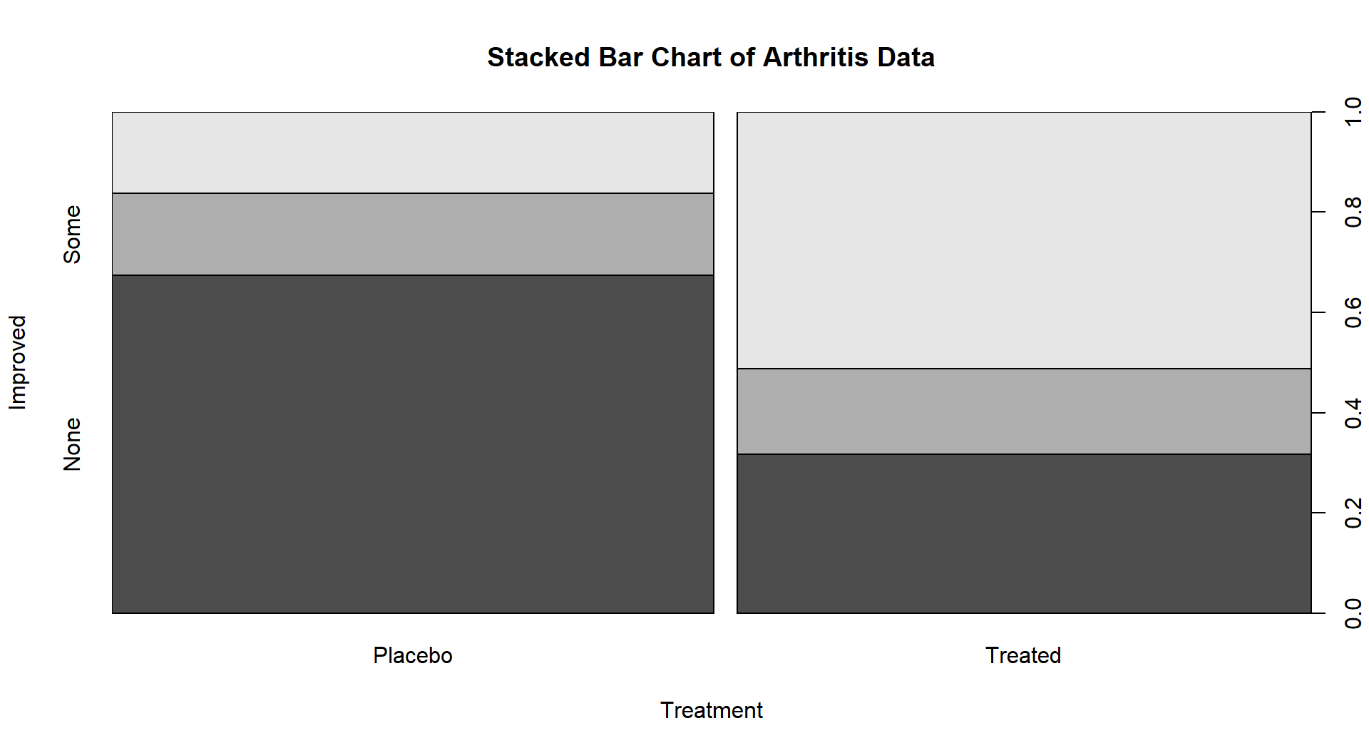
If we revisit our observed results, re-plotted in Figure 2.82 since Figure 2.73 is many pages earlier, knowing that we have strong evidence against the null hypothesis of no difference between Placebo and Treated groups, what can we say about the effectiveness of the arthritis medication? It seems that there is a real and important increase in the proportion of patients getting improvement (Some or Marked). If the differences “looked” smaller, even with a small p-value you⁸⁷ might not recommend someone take the drug…

(ref:fig5-11) Stacked bar chart of the Arthritis data comparing Treated and Placebo.

Figure 2.82: (ref:fig5-11)