- Cover
- Acknowledgments
- 1 Preface
- 2 (R)e-Introduction to statistics
- 2.1 Histograms, boxplots, and density curves
- 2.2 Pirate-plots
- 2.3 Models, hypotheses, and permutations for the two sample mean situation
- 2.4 Permutation testing for the two sample mean situation
- 2.5 Hypothesis testing (general)
- 2.6 Connecting randomization (nonparametric) and parametric tests
- 2.7 Second example of permutation tests
- 2.8 Reproducibility Crisis: Moving beyond p < 0.05, publication bias, and multiple testing issues
- 2.9 Confidence intervals and bootstrapping
- 2.10 Bootstrap confidence intervals for difference in GPAs
- 2.11 Chapter summary
- 2.12 Summary of important R code
- 2.13 Practice problems
- 3 One-Way ANOVA
- 3.1 Situation
- 3.2 Linear model for One-Way ANOVA (cell-means and reference-coding)
- 3.3 One-Way ANOVA Sums of Squares, Mean Squares, and F-test
- 3.4 ANOVA model diagnostics including QQ-plots
- 3.5 Guinea pig tooth growth One-Way ANOVA example
- 3.6 Multiple (pair-wise) comparisons using Tukey’s HSD and the compact letter display
- 3.7 Pair-wise comparisons for the Overtake data
- 3.8 Chapter summary
- 3.9 Summary of important R code
- 3.10 Practice problems
- 4 Two-Way ANOVA
- 4.1 Situation
- 4.2 Designing a two-way experiment and visualizing results
- 4.3 Two-Way ANOVA models and hypothesis tests
- 4.4 Guinea pig tooth growth analysis with Two-Way ANOVA
- 4.5 Observational study example: The Psychology of Debt
- 4.6 Pushing Two-Way ANOVA to the limit: Un-replicated designs and Estimability
- 4.7 Chapter summary
- 4.8 Summary of important R code
- 4.9 Practice problems
- 5 Chi-square tests
- 5.1 Situation, contingency tables, and tableplots
- 5.2 Homogeneity test hypotheses
- 5.3 Independence test hypotheses
- 5.4 Models for R by C tables
- 5.5 Permutation tests for the \(X^2\) statistic
- 5.6 Chi-square distribution for the \(X^2\) statistic
- 5.7 Examining residuals for the source of differences
- 5.8 General protocol for \(X^2\) tests
- 5.9 Political party and voting results: Complete analysis
- 5.10 Is cheating and lying related in students?
- 5.11 Analyzing a stratified random sample of California schools
- 5.12 Chapter summary
- 5.13 Summary of important R commands
- 5.14 Practice problems
- 6 Correlation and Simple Linear Regression
- 6.1 Relationships between two quantitative variables
- 6.2 Estimating the correlation coefficient
- 6.3 Relationships between variables by groups
- 6.4 Inference for the correlation coefficient
- 6.5 Are tree diameters related to tree heights?
- 6.6 Describing relationships with a regression model
- 6.7 Least Squares Estimation
- 6.8 Measuring the strength of regressions: R2
- 6.9 Outliers: leverage and influence
- 6.10 Residual diagnostics – setting the stage for inference
- 6.11 Old Faithful discharge and waiting times
- 6.12 Chapter summary
- 6.13 Summary of important R code
- 6.14 Practice problems
- 7 Simple linear regression inference
- 7.1 Model
- 7.2 Confidence interval and hypothesis tests for the slope and intercept
- 7.3 Bozeman temperature trend
- 7.4 Randomization-based inferences for the slope coefficient
- 7.5 Transformations part I: Linearizing relationships
- 7.6 Transformations part II: Impacts on SLR interpretations: log(y), log(x), & both log(y) & log(x)
- 7.7 Confidence interval for the mean and prediction intervals for a new observation
- 7.8 Chapter summary
- 7.9 Summary of important R code
- 7.10 Practice problems
- 8 Multiple linear regression
- 8.1 Going from SLR to MLR
- 8.2 Validity conditions in MLR
- 8.3 Interpretation of MLR terms
- 8.4 Comparing multiple regression models
- 8.5 General recommendations for MLR interpretations and VIFs
- 8.6 MLR inference: Parameter inferences using the t-distribution
- 8.7 Overall F-test in multiple linear regression
- 8.8 Case study: First year college GPA and SATs
- 8.9 Different intercepts for different groups: MLR with indicator variables
- 8.10 Additive MLR with more than two groups: Headache example
- 8.11 Different slopes and different intercepts
- 8.12 F-tests for MLR models with quantitative and categorical variables and interactions
- 8.13 AICs for model selection
- 8.14 Case study: Forced expiratory volume model selection using AICs
- 8.15 Chapter summary
- 8.16 Summary of important R code
- 8.17 Practice problems
- 9 Case studies
- 9.1 Overview of material covered
- 9.2 The impact of simulated chronic nitrogen deposition on the biomass and N2-fixation activity of two boreal feather moss–cyanobacteria associations
- 9.3 Ants learn to rely on more informative attributes during decision-making
- 9.4 Multi-variate models are essential for understanding vertebrate diversification in deep time
- 9.5 What do didgeridoos really do about sleepiness?
- 9.6 General summary
- References
6.5 Are tree diameters related to tree heights?
In a study at the Upper Flat Creek
study area in the University of Idaho Experimental Forest, a random sample of
\(n=336\) trees was selected from the forest, with measurements recorded on Douglas
Fir, Grand Fir, Western Red
Cedar, and Western Larch trees. The data set called ufc is available from the
spuRs package (Jones et al. 2018) and
contains dbh.cm (tree diameter at 1.37 m from the ground, measured in cm) and
height.m (tree height in meters).
The relationship displayed in
Figure 2.110 is positive,
moderately strong with some curvature and increasing variability as the
diameter increases. There do not appear to be groups in the data set but since
this contains four different types of trees, we would want to revisit this plot
by type of tree.
library(spuRs) #install.packages("spuRs")
data(ufc)
ufc <- as_tibble(ufc)
scatterplot(height.m~dbh.cm, data=ufc, smooth=F, regLine=T)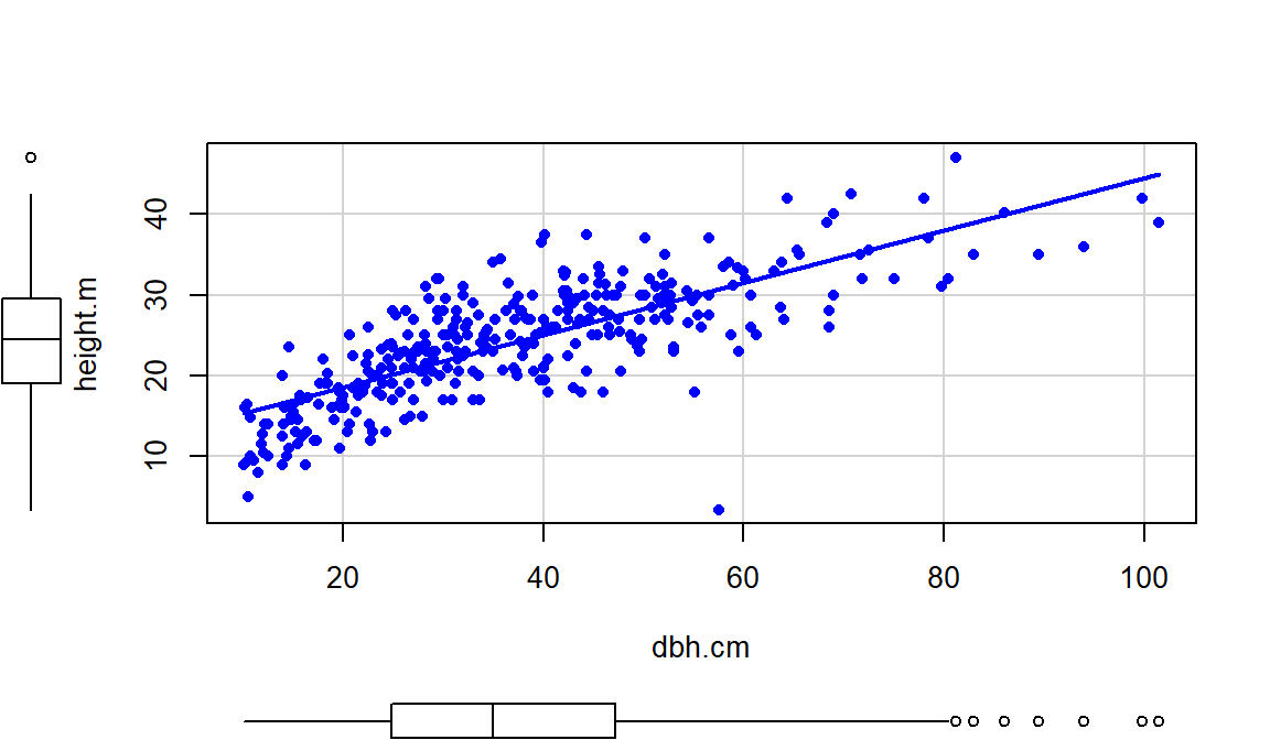
Figure 2.110: Scatterplot of tree heights (m) vs tree diameters (cm).
Of particular interest is an observation with a diameter around 58 cm and a height of less than 5 m. Observing a tree with a diameter around 60 cm is not unusual in the data set, but none of the other trees with this diameter had heights under 15 m. It ends up that the likely outlier is in observation number 168 and because it is so unusual it likely corresponds to either a damaged tree or a recording error.
## # A tibble: 1 x 5
##    plot  tree species dbh.cm height.m
##   <int> <int> <fct>    <dbl>    <dbl>
## 1    67     6 WL        57.5      3.4
With the outlier in the data set, the correlation is 0.77 and without it, the correlation increases to 0.79. The removal does not create a big change because the data set is relatively large and the diameter value is close to the mean of the \(x\text{'s}\)97 but it has some impact on the strength of the correlation.
## [1] 0.7699552## [1] 0.7912053With the outlier included, the bootstrap 95% confidence interval goes from 0.702 to 0.820 – we are 95% confident that the true correlation between diameter and height in the population of trees is between 0.708 and 0.819. When the outlier is dropped from the data set, the 95% bootstrap CI is 0.753 to 0.826, which shifts the lower endpoint of the interval up, reducing the width of the interval from 0.111 to 0.073. In other words, the uncertainty regarding the value of the population correlation coefficient is reduced. The reason to remove the observation is that it is unusual based on the observed pattern, which implies an error in data collection or sampling from a population other than the one used for the other observations and, if the removal is justified, it helps us refine our inferences for the population parameter. But measuring the linear relationship in these data where there is a clear curve violates one of our assumptions of using these methods – we’ll see some other ways of detecting this issue in Section 6.10 and we’ll try to “fix” this example using transformations in the Chapter ??.
(ref:fig6-12) Bootstrap distributions of the correlation coefficient for the full data set (top) and without potential outlier included (bottom) with observed correlation (bold line) and bounds for the 95% confidence interval (dashed lines). Notice the change in spread of the bootstrap distributions as well as the different centers.
## [1] 0.7699552set.seed(208)
par(mfrow=c(2,1))
B <- 1000
Tstar <- matrix(NA, nrow=B)
for (b in (1:B)){
Tstar[b] <- cor(dbh.cm~height.m, data=resample(ufc))
}
quantiles <- qdata(Tstar, c(.025,.975)) #95% Confidence Interval
quantiles## quantile p
## 2.5% 0.7075771 0.025
## 97.5% 0.8190283 0.975hist(Tstar, labels=T, xlim=c(0.6,0.9), ylim=c(0,275),
main="Bootstrap distribution of correlation with all data")
abline(v=Tobs, col="red", lwd=3)
abline(v=quantiles$quantile, col="blue", lty=2, lwd=3)
Tobs <- cor(dbh.cm~height.m, data=ufc[-168,]); Tobs## [1] 0.7912053Tstar <- matrix(NA, nrow=B)
for (b in (1:B)){
Tstar[b] <- cor(dbh.cm~height.m, data=resample(ufc[-168,]))
}
quantiles <- qdata(Tstar, c(.025,.975)) #95% Confidence Interval
quantiles## quantile p
## 2.5% 0.7532338 0.025
## 97.5% 0.8259416 0.975hist(Tstar, labels=T, xlim=c(0.6,0.9), ylim=c(0,275),
main= "Bootstrap distribution of correlation without outlier")
abline(v=Tobs, col="red", lwd=3)
abline(v=quantiles$quantile, col="blue", lty=2, lwd=3)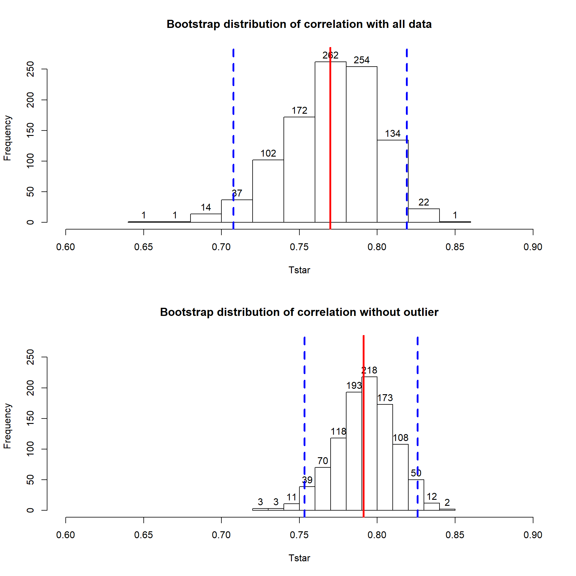
Figure 2.111: (ref:fig6-12)
References
Jones, Owen, Robert Maillardet, Andrew Robinson, Olga Borovkova, and Steven Carnie. 2018. SpuRs: Functions and Datasets for "Introduction to Scientific Programming and Simulation Using R". https://CRAN.R-project.org/package=spuRs.