8.9 Different intercepts for different groups: MLR with indicator variables

One of the implicit assumptions up to this point was that the models were being applied to a single homogeneous population. In many cases, we take a sample from a population but that overall group is likely a combination of individuals from different sub-populations. For example, the SAT study was interested in all students at the university but that contains the obvious sub-populations based on the gender of the students. It is dangerous to fit MLR models across subpopulations but we can also use MLR models to address more sophisticated research questions by comparing groups. We will be able to compare the intercepts (mean levels) and the slopes to see if they differ between the groups. For example, does the relationship between the SATV and FYGPA differ for male and female students? We can add the grouping information to the scatterplot of FYGPA vs SATV (Figure 2.167) and consider whether there is visual evidence of a difference in the slope and/or intercept between the two groups, with men coded¹²⁶ as 1 and women coded as 2. Code below changes this variable to GENDER with more explicit labels, even though they might not be correct and the students were likely forced to choose one or the other.

It appears that the slope for females might be larger (steeper) in this relationship than it is for males. So increases in SAT Verbal percentiles for females might have more of an impact on the average first year GPA. We’ll handle this sort of situation in Section 8.11, where we will formally consider how to change the slopes for different groups. In this section, we develop new methods needed to begin to handle these situations and explore creating models that assume the same slope coefficient for all groups but allow for different y-intercepts. This material ends up resembling what we did for the Two-Way ANOVA additive model.

The results for SATV contrast with Figure 2.168 for the relationship between first year college GPA and SATM percentile by gender of the students. The lines for the two groups appear to be mostly parallel and just seem to have different y-intercepts. In this section, we will learn how we can use our MLR techniques to fit a model to the entire data set that allows for different y-intercepts. The real power of this idea is that we can then also test whether the different groups have different y-intercepts – whether the shift between the groups is “real”. In this example, it appears to suggest that females generally have slightly higher GPAs than males, on average, but that an increase in SATM has about the same impact on GPA for both groups. If this difference in y-intercepts is not “real”, then there appears to be no difference between the sexes in their relationship between SATM and GPA and we can safely continue using a model that does not differentiate the two groups. We could also just subset the data set and do two analyses, but that approach will not allow us to assess whether things are “really” different between the two groups.

satGPA$GENDER <- factor(satGPA$sex) #Make 1,2 coded sex into factor GENDER
levels(satGPA$GENDER) <- c("MALE", "FEMALE") #Make category names clear but names might be wrong
scatterplot(FYGPA~SATV|GENDER, lwd=3, data=satGPA, smooth=F,
            main="Scatterplot of GPA vs SATV by Sex")
scatterplot(FYGPA~SATM|GENDER, lwd=3, data=satGPA, smooth=F,
            main="Scatterplot of GPA vs SATM by Sex")

To fit one model to a data set that contains multiple groups, we need a way of entering categorical variable information in an MLR model. Regression models require quantitative predictor variables for the \(x\text{'s}\) so we can’t directly enter the text coded information on the gender of the students into the regression model since it contains “words” and how can multiply a word times a slope coefficient. To be able to put in “numbers” as predictors, we create what are called indicator variables¹²⁷ that are made up of 0s and 1s, with the 0 reflecting one category and 1 the other, changing depending on the category of the individual in that row of the data set. The lm function does this whenever a factor variable is used as an explanatory variable. It sets up the indicator variables using a baseline category (which gets coded as a 0) and the deviation category for the other level of the variable (which gets coded as a 1). We can see how this works by exploring what happens when we put GENDER into our lm with SATM, after first making sure it is categorical using the factor function and making the factor levels explicit instead of 1s and 2s.

satGPA$GENDER <- factor(satGPA$sex) #Make 1,2 coded sex into factor GENDER
levels(satGPA$GENDER) <- c("MALE", "FEMALE") #Make category names clear but names might be wrong
SATGENDER1 <- lm(FYGPA~SATM+GENDER, data=satGPA) #Fit lm with SATM and SEX
summary(SATGENDER1)

## 
## Call:
## lm(formula = FYGPA ~ SATM + GENDER, data = satGPA)
## 
## Residuals:
##      Min       1Q   Median       3Q      Max 
## -2.42124 -0.42363  0.01868  0.46540  1.66397 
## 
## Coefficients:
##              Estimate Std. Error t value Pr(>|t|)
## (Intercept)   0.21589    0.14858   1.453    0.147
## SATM          0.03861    0.00258  14.969  < 2e-16
## GENDERFEMALE  0.31322    0.04360   7.184 1.32e-12
## 
## Residual standard error: 0.6667 on 997 degrees of freedom
## Multiple R-squared:  0.1917, Adjusted R-squared:  0.1901 
## F-statistic: 118.2 on 2 and 997 DF,  p-value: < 2.2e-16

Figure 2.167: Plot of FYGPA vs SATV by Sex of students.

Figure 2.168: Plot of FYGPA vs SATM by Sex of students.

The GENDER row contains information that the linear model chose MALE as the baseline category and FEMALE as the deviation category since MALE does not show up in the output. To see what lm is doing for us when we give it a two-level categorical variable, we can create our own “numerical” predictor that is 0 for males and 1 for females that we called GENDERINDICATOR, displayed for the first 10 observations:

# Convert logical to 0 for male, 1 for female
satGPA$GENDERINDICATOR <- as.numeric(satGPA$GENDER=="FEMALE") 
# Explore first few observations
head(tibble(GENDER=satGPA$GENDER, GENDERINDICATOR=satGPA$GENDERINDICATOR), 10) 

## # A tibble: 10 x 2
##    GENDER GENDERINDICATOR
##    <fct>            <dbl>
##  1 MALE                 0
##  2 FEMALE               1
##  3 FEMALE               1
##  4 MALE                 0
##  5 MALE                 0
##  6 FEMALE               1
##  7 MALE                 0
##  8 MALE                 0
##  9 FEMALE               1
## 10 MALE                 0

We can define the indicator variable more generally by calling it \(I_{\text{Female},i}\) to denote that it is an indicator \((I)\) that takes on a value of 1 for observations in the category Female and 0 otherwise (Male) – changing based on the observation (\(i\)). Indicator variables, once created, are quantitative variables that take on values of 0 or 1 and we can put them directly into linear models with other \(x\text{'s}\) (quantitative or categorical). If we replace the categorical GENDER variable with our quantitative GENDERINDICATOR and re-fit the model, we get:

SATGENDER2 <- lm(FYGPA~SATM+GENDERINDICATOR, data=satGPA)
summary(SATGENDER2)

## 
## Call:
## lm(formula = FYGPA ~ SATM + GENDERINDICATOR, data = satGPA)
## 
## Residuals:
##      Min       1Q   Median       3Q      Max 
## -2.42124 -0.42363  0.01868  0.46540  1.66397 
## 
## Coefficients:
##                 Estimate Std. Error t value Pr(>|t|)
## (Intercept)      0.21589    0.14858   1.453    0.147
## SATM             0.03861    0.00258  14.969  < 2e-16
## GENDERINDICATOR  0.31322    0.04360   7.184 1.32e-12
## 
## Residual standard error: 0.6667 on 997 degrees of freedom
## Multiple R-squared:  0.1917, Adjusted R-squared:  0.1901 
## F-statistic: 118.2 on 2 and 997 DF,  p-value: < 2.2e-16

This matches all the previous lm output except that we didn’t get any information on the categories used since lm didn’t know that GENDERINDICATOR was anything different from other quantitative predictors.

Now we want to think about what this model means. We can write the estimated model as

\[\widehat{\text{FYGPA}}_i = 0.216 + 0.0386\cdot\text{SATM}_i + 0.313I_{\text{Female},i}\ .\]

When we have a male observation, the indicator takes on a value of 0 so the 0.313 drops out of the model, leaving an SLR just in terms of SATM. For a female student, the indicator is 1 and we add 0.313 to the previous y-intercept. The following works this out step-by-step, simplifying the MLR into two SLRs:

• Simplified model for Males (plug in a 0 for \(I_{\text{Female},i}\)):

  • \(\widehat{\text{FYGPA}}_i = 0.216 + 0.0386\cdot\text{SATM}_i + 0.313*0 = 0.216 + 0.0386\cdot\text{SATM}_i\)

• Simplified model for Females (plug in a 1 for \(I_{\text{Female},i}\)):

  • \(\widehat{\text{FYGPA}}_i = 0.216 + 0.0386\cdot\text{SATM}_i + 0.313*1\)

  • \(= 0.216 + 0.0386\cdot\text{SATM}_i + 0.313\) (combine “like” terms to simplify the equation)

  • \(= 0.529 + 0.0386\cdot\text{SATM}_i\)

In this situation, we then end up with two SLR models that relate SATM to GPA, one model for males \((\widehat{\text{FYGPA}}_i= 0.216 + 0.0386\cdot\text{SATM}_i)\) and one for females \((\widehat{\text{FYGPA}}_i= 0.529 + 0.0386\cdot\text{SATM}_i)\). The only difference between these two models is in the y-intercept, with the female model’s y-intercept shifted up from the male y-intercept by 0.313. And that is what adding indicator variables into models does in general¹²⁸ – it shifts the intercept up or down from the baseline group (here selected as males) to get a new intercept for the deviation group (here females).

To make this visually clearer, Figure 2.169 contains the regression lines that were estimated for each group. For any SATM, the difference in the groups is the 0.313 coefficient from the GENDERFEMALE or GENDERINDICATOR row of the model summaries. For example, at SATM=50, the difference in terms of predicted average first year GPAs between males and females is displayed as a difference between 2.15 and 2.46. This model assumes that the slope on SATM is the same for both groups except that they are allowed to have different y-intercepts, which is reasonable here because we saw approximately parallel relationships for the two groups in Figure 2.168.

(ref:fig8-19) Plot of estimated model for FYGPA vs SATM by GENDER of students (female line is thicker dark line). Dashed lines aid in seeing the consistent vertical difference of 0.313 in the two estimated lines based on the model containing a different intercept for each group.

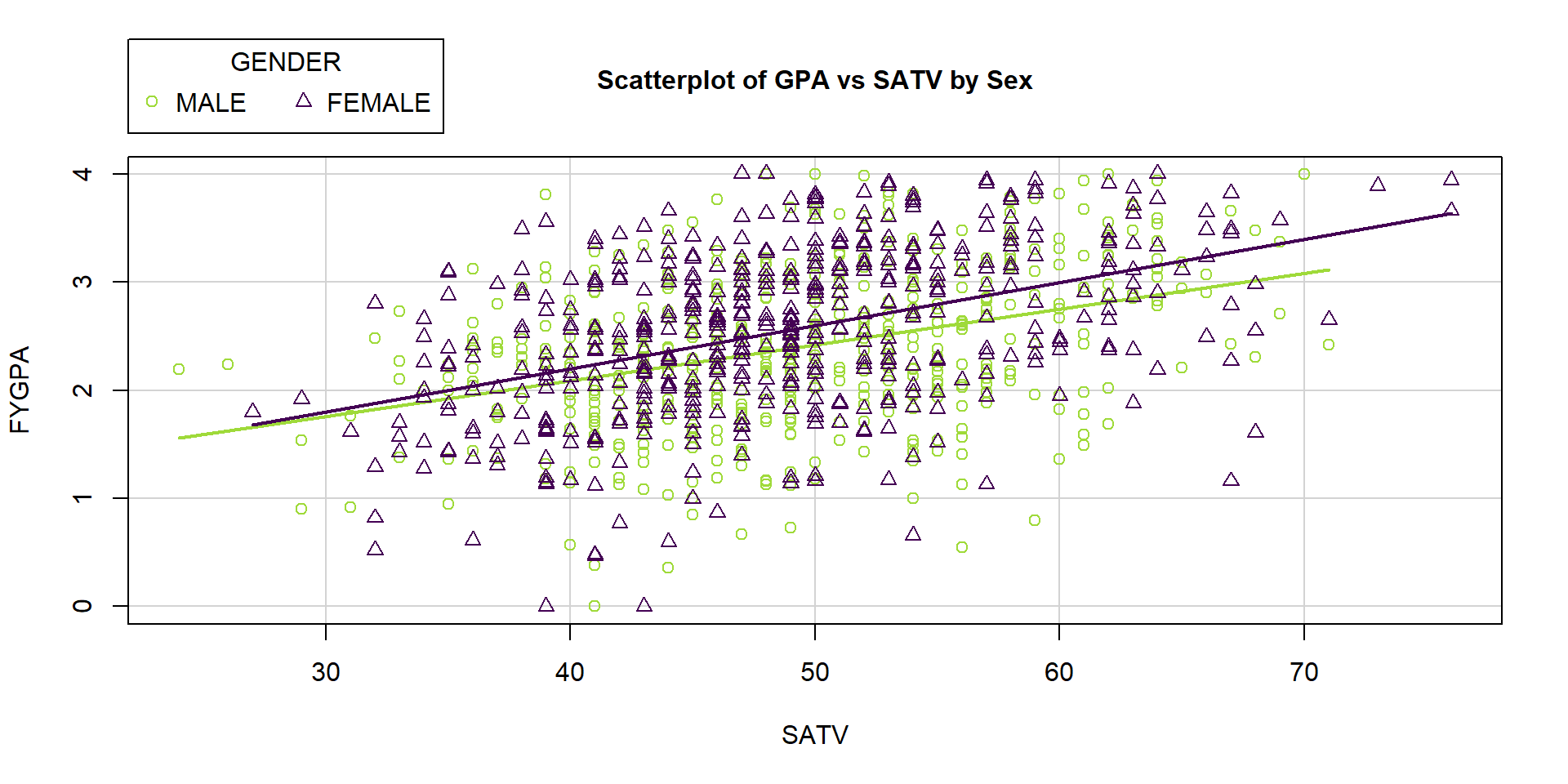
Figure 2.169: (ref:fig8-19)

Remember that lm selects baseline categories typically based on the alphabetical order of the levels of the categorical variable when it is created unless the reorder function is used to change the order. Here, the GENDER variable started with a coding of 1 and 2 and retained that order even with the recoding of levels that we created to give it more explicit names. Because we allow lm to create indicator variables for us, the main thing you need to do is explore the model summary and look for the hint at the baseline level that is not displayed after the name of the categorical variable.

We can also work out the impacts of adding an indicator variable to the model in general in the theoretical model with a single quantitative predictor \(x_i\) and indicator \(I_i\). The model starts as

\[y_i=\beta_0+\beta_1x_i + \beta_2I_i + \varepsilon_i\ .\]

Again, there are two versions:

• For any observation \(i\) in the baseline category, \(I_i=0\) and the model is \(y_i=\beta_0+\beta_1x_i + \varepsilon_i\).

• For any observation \(i\) in the non-baseline (deviation) category, \(I_i=1\) and the model simplifies to \(y_i=(\beta_0+\beta_2)+\beta_1x_i + \varepsilon_i\).

  • This model has a y-intercept of \(\beta_0+\beta_2\).

The interpretation and inferences for \(\beta_1\) resemble the work with any MLR model, noting that these results are “controlled for”, “adjusted for”, or “allowing for differences based on” the categorical variable in the model. The interpretation of \(\beta_2\) is as a shift up or down in the y-intercept for the model that includes \(x_i\). When we make term-plots in a model with a quantitative and additive categorical variable, the two reported model components match with the previous discussion – the same estimated term from the quantitative variable for all observations and a shift to reflect the different y-intercepts in the two groups. In Figure 2.170, the females are estimated to be that same 0.313 points higher on first year GPA. The males have a mean GPA slightly above 2.3 which is the predicted GPA for the average SATM percentile for a male (remember that we have to hold the other variable at its mean to make each term-plot). When making the SATM term-plot, the categorical variable is held at the most frequently occurring value (modal category) in the data set, which is for males in this data set.

(ref:fig8-20) Term-plots for the estimated model for \(\text{FYGPA}\sim\text{SATM} + \text{GENDER}\).

tally(GENDER~1, data=satGPA)

##         1
## GENDER     1
##   MALE   516
##   FEMALE 484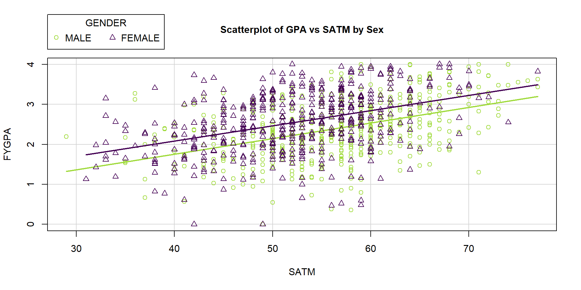

plot(allEffects(SATGENDER1))

Figure 2.170: (ref:fig8-20)

The model summary and confidence intervals provide some potential interesting inferences in these models. Again, these are just applications of MLR methods we have already seen except that the definition of one of the variables is “different” using the indicator coding idea. For the same model, the GENDER coefficient can be used to generate inferences for differences in the mean the groups, controlling for their SATM scores.

##                Estimate Std. Error t value Pr(>|t|)
## GENDERFEMALE    0.31322    0.04360   7.184 1.32e-12

Testing the null hypothesis that \(H_0: \beta_2=0\) vs \(H_A: \beta_2\ne 0\) using our regular \(t\)-test provides the opportunity to test for a difference in intercepts between the groups. In this situation, the test statistic is \(t=7.184\) and, based on a \(t_{997}\)-distribution if the null is true, the p-value is \(<0.0001\). We have very strong evidence against the null hypothesis that there is no difference in the true y-intercept in a SATM model for first year college GPA between males and females, so we would conclude that there is difference in their true mean GPA levels controlled for SATM. The confidence interval is also informative:

confint(SATGENDER1)

##                    2.5 %     97.5 %
## (Intercept)  -0.07566665 0.50744709
## SATM          0.03355273 0.04367726
## GENDERFEMALE  0.22766284 0.39877160

We are 95% confident that the true mean GPA for females is between 0.228 and 0.399 points higher than for males, after adjusting for the SATM in the population of students. If we had subset the data set and fit two SLRs, we could have obtained the same simplified regression models but we never could have performed inferences for the differences between the two groups without putting all the observations together in one model and then assessing those differences with targeted coefficients. We also would not be able to get an estimate of their common slope for SATM, after adjusting for differences in the intercept for each group.